19. Simulated Method of Moments Estimation#
This chapter describes the simulated method of moments (SMM) estimation method. All data and images from this chapter can be found in the data directory (./data/smm/) and images directory (./images/smm/) for the GitHub repository for this online book.
19.1. The SMM estimator#
Simulated method of moments (SMM) is analogous to the generalized method of moments (GMM) estimator. SMM could really be thought of as a particular type of GMM estimator. The SMM estimator chooses a vector of model parameters \(\theta\) to make simulated model moments match data moments. Seminal papers developing SMM are [McFadden, 1989], [Lee and Ingram, 1991], and [Duffie and Singleton, 1993]. Good textbook treatments of SMM are found in [Adda and Cooper, 2003], (pp. 87-100) and [Davidson and MacKinnon, 2004], (pp. 383-394).
Let the data be represented, in general, by \(x\). This could have many variables, and it could be cross-sectional or time series. We define the estimation problem as one in which we want to model the data \(x\) using some parameterized model \(g(x|\theta)\) in which \(\theta\) is a \(K\times 1\) vector of parameters.
In the Maximum Likelihood Estimation chapter, we used data \(x\) and model parameters \(\theta\) to maximize the likelihood of drawing that data \(x\) from the model given parameters \(\theta\),
where \(f(x_i|\theta)\) is the likelihood of seeing observation \(x_i\) in the data \(x\) given vector of parameters \(\theta\).
In the Generalized Method of Moments Estimation chapter, we used data \(x\) and the \(K\times 1\) vector of model parameters \(\theta\) to minimize the distance between the vector of \(R\geq K\) model moments \(m(x|\theta)\) and data moments \(m(x)\),
where,
and,
The following difficulties can arise with GMM making it not possible or very difficult.
The model moment function \(m(x|\theta)\) is not known analytically.
The data moments you are trying to match come from another model (indirect inference, see [Smith, 2020]).
The model moments \(m(x|\theta)\) are derived from latent variables that are not observed by the modeler. You only have moments, not the underlying data. See [Laroque and Salanié, 1993].
The model moments \(m(x|\theta)\) are derived from censored variables that are only partially observed by the modeler.
The model moments \(m(x|\theta)\) are just difficult to derive analytically. Examples include moments that include multiple integrals over nonlinear functions as in [McFadden, 1989].
SMM estimation is simply to simulate the model data \(S\) times, and use the average values of the moments from the simulated data as the estimator for the model moments. Let \(\tilde{x}\equiv\{\tilde{x}_1,\tilde{x}_2,...\tilde{x}_s,...\tilde{x}_S\}\) be the \(S\) simulations of the model data. And let the maximization problem in (19.8) be characterized by \(R\) average moments across simulations, where \(\hat{m}_r\) is the average value of the \(r\)th moment across the \(S\) simulations where,
and
Once we have an estimate of the vector of \(R\) average model moments \(\hat{m}\left(\tilde{x}|\theta\right)\) from our \(S\) simulations, SMM estimation is very similar to our presentation of GMM in Generalized Method of Moments Estimation. The SMM approach of estimating the \(K\times 1\) parameter vector \(\hat{\theta}_{SMM}\) is to choose vector \(\theta\) to minimize some distance measure of the \(R\) data moments \(m(x)\) from the \(R\) simulated average model moments \(\hat{m}(\tilde{x}|\theta)\).
The distance measure \(||\hat{m}(\tilde{x}|\theta)-m(x)||\) can be any kind of norm. But it is important to recognize that your estimates \(\hat{\theta}_{SMM}\) will be dependent on what distance measure (norm) you choose. The most widely studied and used distance metric in GMM and SMM estimation is the \(L^2\) norm or the sum of squared errors in moments.
Define the moment error vector \(e(\tilde{x},x|\theta)\) as the \(R\times 1\) vector of average moment error functions \(e_r(\tilde{x},x|\theta)\) of the \(r\)th average moment error.
We can define the \(r\)th average moment error as the percent difference in the average simulated \(r\)th moment value \(\hat{m}_r(\tilde{x}|\theta)\) from the \(r\)th data moment \(m_r(x)\).
It is important that the error function \(e_r(\tilde{x},x|\theta)\) be a percent deviation of the moments, although this will not work if the data moments are 0 or can be either positive or negative. This percent change transformation puts all the moments in the same units, which helps make sure that no moments receive unintended weighting simply due to its units. This ensures that the problem is scaled properly and will suffer from as little as possible ill conditioning.
In this case, the SMM estimator is the following,
where \(W\) is a \(R\times R\) weighting matrix in the criterion function. For now, think of this weighting matrix as the identity matrix. But we will show in Section The Weighting Matrix (W) a more optimal weighting matrix. We call the quadratic form expression \(e(\tilde{x},x|\theta)^T \, W \, e(\tilde{x},x|\theta)\) the criterion function because it is a strictly positive scalar that is the object of the minimization in the SMM problem statement. The \(R\times R\) weighting matrix \(W\) in the criterion function allows the econometrician to control how each moment is weighted in the minimization problem. For example, an \(R\times R\) identity matrix for \(W\) would give each moment equal weighting, and the criterion function would be a simply sum of squared percent deviations (errors). Other weighting strategies can be dictated by the nature of the problem or model.
One last item to emphasize with SMM, which we will highlight in the examples in this chapter, is that the errors that are drawn for the \(S\) simulations of the model must be drawn only once so that the minimization problem for estimating \(\hat{\theta}_{SMM}\) does not have the underlying sampling changing for each guess of a value of \(\theta\). Put more simply, you want the random draws for all the simulations to be held constant so that the only thing changing in the minimization problem is the value of the vector of parameters \(\theta\).
19.2. The Weighting Matrix (W)#
In the SMM criterion function in the problem statement above, some weighting matrices \(W\) produce precise estimates while others produce poor estimates with large variances. We want to choose the optimal weighting matrix \(W\) with the smallest possible asymptotic variance. This is an efficient or optimal SMM estimator. The optimal weighting matrix is the inverse variance covariance matrix of the moments at the optimal moments,
where \(\Omega(\tilde{x},x|\theta)\) is the variance covariance matrix of the moment condition errors \(e(\tilde{x},x|\theta)\). The intuition for using the inverse variance covariance matrix \(\Omega^{-1}\) as the optimal weighting matrix is the following. You want to downweight moments that have a high variance, and you want to weight more heavily the moments that are generated more precisely.
Notice that this definition of the optimal weighting matrix is circular. \(W^{opt}\) is a function of the SMM estimates \(\hat{\theta}_{SMM}\), but the optimal weighting matrix is used in the estimation of \(\hat{\theta}_{SMM}\). This means that one has to use some kind of iterative fixed point method to find the true optimal weighting matrix \(W^{opt}\). Below are some examples of weighting matrices to use.
19.2.1. The identity matrix (W=I)#
Many times, you can get away with just using the identity matrix as your weighting matrix \(W = I\). This changes the criterion function to a simple sum of squared error functions such that each moment has the same weight.
If the problem is well conditioned and well identified, then your SMM estimates \(\hat{\theta}_{SMM}\) will not be greatly affected by this simplest of weighting matrices.
19.2.2. Two-step variance-covariance estimator of W#
The most common method of estimating the optimal weighting matrix for SMM estimates is the two-step variance covariance estimator. The name “two-step” refers to the two steps used to get the weighting matrix.
The first step is to estimate the SMM parameter vector \(\hat{\theta}_{1,SMM}\) using the simple identity matrix as the weighting matrix \(W = I\).
Because we are simulating data, we can generate an estimator for the variance covariance matrix of the moment error vector \(\hat{\Omega}\) using just the simulated data moments and the data moments. This \(E(\tilde{x},x|\theta)\) matrix represents the contribution of the \(s\)th simulated moment to the \(r\)th moment error. Define \(E(\tilde{x},x|\theta)\) as the \(R\times S\) matrix of moment error functions from each simulation,
where \(m_r(x)\) is the \(r\)th data moment which is constant across each row, and \(m_r(\tilde{x}_s|\theta)\) is the \(r\)th model moment from the \(s\)th simulation which are changing across each row. When the errors are percent deviations, the \(E(\tilde{x},x|\theta)\) matrix is the following,
where the denominator of the percentage deviation or baseline is the model moment that does not change. We use the \(E(\tilde{x},x|\theta)\) data matrix and the Step 1 SMM estimate \(e(x|\hat{\theta}_{1,SMM})\) to get a new \(R\times R\) estimate of the variance covariance matrix.
This is simply saying that the \((r,s)\)-element of the \(R\times R\) estimator of the variance-covariance matrix of the moment vector is the following.
The optimal weighting matrix is the inverse of the two-step variance covariance matrix.
Lastly, re-estimate the SMM estimator using the optimal two-step weighting matrix \(\hat{W}^{2step}\).
\(\hat{\theta}_{2, SMM}\) is called the two-step SMM estimator.
19.2.3. Iterated variance-covariance estimator of W#
The truly optimal weighting matrix \(W^{opt}\) is the iterated variance-covariance estimator of \(W\). This procedure is to just repeat the process described in the two-step SMM estimator until the estimated weighting matrix no longer significantly changes between iterations. Let \(i\) index the \(i\)th iterated SMM estimator,
and the \((i+1)\)th estimate of the optimal weighting matrix is defined as the following.
The iterated SMM estimator \(\hat{\theta}_{it,SMM}\) is the \(\hat{\theta}_{i,SMM}\) such that \(\hat{W}_{i+1}\) is very close to \(\hat{W}_{i}\) for some distance metric (norm).
19.2.4. Newey-West consistent estimator of \(\Omega\) and W#
The Newey-West estimator of the optimal weighting matrix and variance covariance matrix is consistent in the presence of heteroskedasticity and autocorrelation in the data (See [Newey and West, 1987]). [Adda and Cooper, 2003] (p. 82) have a nice exposition of how to compute the Newey-West weighting matrix \(\hat{W}_{nw}\). The asymptotic representation of the optimal weighting matrix \(\hat{W}^{opt}\) is the following:
The Newey-West consistent estimator of \(\hat{W}^{opt}\) is:
where
Of course, for autocorrelation, the subscript \(i\) can be changed to \(t\).
19.3. Variance-Covariance Estimator of \(\hat{\theta}\)#
Let the parameter vector \(\theta\) have length \(K\) such that \(K\) parameters are being estimated. The estimated \(K\times K\) variance-covariance matrix \(\hat{\Sigma}\) of the estimated parameter vector \(\hat{\theta}_{SMM}\) is different from the \(R\times R\) variance-covariance matrix \(\hat{\Omega}\) of the \(R\times 1\) moment vector \(e(\tilde{x},x|\theta)\) from the previous section.
Recall that each element of \(e(\tilde{x},x|\theta)\) is an average moment error across all simulations. \(\hat{\Omega}\) from the previous section is the \(R\times R\) variance-covariance matrix of the \(R\) moment errors used to identify the \(K\) parameters \(\theta\) to be estimated. The estimated variance-covariance matrix \(\hat{\Sigma}\) of the estimated parameter vector is a \(K\times K\) matrix. We say the model is exactly identified if \(K = R\) (number of parameters \(K\) equals number of moments \(R\)). We say the model is overidentified if \(K<R\). We say the model is not identified or underidentified if \(K>R\).
Similar to the inverse Hessian estimator of the variance-covariance matrix of the maximum likelihood estimator from the Maximum Likelihood Estimation chapter, the SMM variance-covariance matrix is related to the derivative of the criterion function with respect to each parameter. The intuition is that if the second derivative of the criterion function with respect to the parameters is large, there is a lot of curvature around the criterion minimizing estimate. In other words, the parameters of the model are precisely estimated. The inverse of the Hessian matrix will be small.
Define \(R\times K\) matrix \(d(\tilde{x},x|\theta)\) as the Jacobian matrix of derivatives of the \(R\times 1\) error vector \(e(\tilde{x},x|\theta)\) from (19.9).
The SMM estimates of the parameter vector \(\hat{\theta}_{SMM}\) are assymptotically normal. If \(\theta_0\) is the true value of the parameters, then the following holds,
where \(W\) is the optimal weighting matrix from the SMM criterion function. The SMM estimator for the variance-covariance matrix \(\hat{\Sigma}_{SMM}\) of the parameter vector \(\hat{\theta}_{SMM}\) is the following.
In the examples below, we will use a finite difference method to compute numerical versions of the Jacobian matrix \(d(\tilde{x},x|\theta)\). The following is a first-order forward finite difference numerical approximation of the first derivative of a function.
The following is a centered second-order finite difference numerical approximation of the derivative of a function. (See BYU ACME numerical differentiation lab for more details.)
19.4. Code Examples#
In this section, we will use SMM to estimate parameters of the models from the Maximum Likelihood Estimation chapter and from the Generalized Method of Moments Estimation chapter.
19.4.1. Fitting a truncated normal to intermediate macroeconomics test scores#
Let’s revisit the problem from the MLE and GMM notebooks of fitting a truncated normal distribution to intermediate macroeconomics test scores. The data are in the text file Econ381totpts.txt. Recall that these test scores are between 0 and 450. Figure 19.1 below shows a histogram of the data, as well as three truncated normal PDF’s with different values for \(\mu\) and \(\sigma\). The black line is the maximum likelihood estimate of \(\mu\) and \(\sigma\) of the truncated normal pdf from the Maximum Likelihood Estimation chapter. The red, green, and black lines are just the PDF’s of two “arbitrarily” chosen combinations of the truncated normal parameters \(\mu\) and \(\sigma\).[1]
Show code cell source
# Import the necessary libraries
import numpy as np
import scipy.stats as sts
import requests
import matplotlib.pyplot as plt
from mpl_toolkits.mplot3d import Axes3D


def trunc_norm_pdf(xvals, mu, sigma, cut_lb=None, cut_ub=None):
    '''
    --------------------------------------------------------------------
    Generate pdf values from the normal pdf with mean mu and standard
    deviation sigma. If the cutoff is given, then the PDF values are
    inflated upward to reflect the zero probability on values above the
    cutoff. If there is no cutoff given, this function does the same
    thing as sp.stats.norm.pdf(x, loc=mu, scale=sigma).
    --------------------------------------------------------------------
    INPUTS:
    xvals  = (N,) vector, values of the normally distributed random
             variable
    mu     = scalar, mean of the normally distributed random variable
    sigma  = scalar > 0, standard deviation of the normally distributed
             random variable
    cut_lb = scalar or string, ='None' if no cutoff is given, otherwise
             is scalar lower bound value of distribution. Values below
             this value have zero probability
    cut_ub = scalar or string, ='None' if no cutoff is given, otherwise
             is scalar upper bound value of distribution. Values above
             this value have zero probability

    OTHER FUNCTIONS AND FILES CALLED BY THIS FUNCTION: None

    OBJECTS CREATED WITHIN FUNCTION:
    prob_notcut = scalar
    pdf_vals = (N,) vector, normal PDF values for mu and sigma
               corresponding to xvals data

    FILES CREATED BY THIS FUNCTION: None

    RETURNS: pdf_vals
    --------------------------------------------------------------------
    '''
    if cut_ub == 'None' and cut_lb == 'None':
        prob_notcut = 1.0
    elif cut_ub == 'None' and cut_lb != 'None':
        prob_notcut = 1.0 - sts.norm.cdf(cut_lb, loc=mu, scale=sigma)
    elif cut_ub != 'None' and cut_lb == 'None':
        prob_notcut = sts.norm.cdf(cut_ub, loc=mu, scale=sigma)
    elif cut_ub != 'None' and cut_lb != 'None':
        prob_notcut = (sts.norm.cdf(cut_ub, loc=mu, scale=sigma) -
                       sts.norm.cdf(cut_lb, loc=mu, scale=sigma))

    pdf_vals    = ((1/(sigma * np.sqrt(2 * np.pi)) *
                    np.exp( - (xvals - mu)**2 / (2 * sigma**2))) /
                    prob_notcut)

    return pdf_vals


# Download and save the data file Econ381totpts.txt as NumPy array
url = ('https://raw.githubusercontent.com/OpenSourceEcon/CompMethods/' +
       'main/data/smm/Econ381totpts.txt')
data_file = requests.get(url, allow_redirects=True)
open('../../../data/smm/Econ381totpts.txt', 'wb').write(data_file.content)
if data_file.status_code == 200:
    # Load the downloaded data into a NumPy array
    data = np.loadtxt('../../../data/smm/Econ381totpts.txt')
else:
    print('Error downloading the file')

num_bins = 30
count, bins, ignored = plt.hist(
    data, num_bins, density=True, edgecolor='k', label='data'
)
plt.title('Intermediate macro scores: 2011-2012', fontsize=20)
plt.xlabel(r'Total points')
plt.ylabel(r'Percent of scores')
plt.xlim([0, 550])  # This gives the xmin and xmax to be plotted"

# Plot smooth line with distribution 1
dist_pts = np.linspace(0, 450, 500)
mu_1 = 300
sig_1 = 30
plt.plot(dist_pts, trunc_norm_pdf(dist_pts, mu_1, sig_1, 0, 450),
         linewidth=2, color='red', label=f"$\mu$={mu_1},$\sigma$={sig_1}")

# Plot smooth line with distribution 2
mu_2 = 400
sig_2 = 70
plt.plot(dist_pts, trunc_norm_pdf(dist_pts, mu_2, sig_2, 0, 450),
         linewidth=2, color='green', label=f"$\mu$={mu_2},$\sigma$={sig_2}")

# Plot smooth line with distribution 3
mu_3 = 558
sig_3 = 176
plt.plot(dist_pts, trunc_norm_pdf(dist_pts, mu_3, sig_3, 0, 450),
         linewidth=2, color='black', label=f"$\mu$={mu_3},$\sigma$={sig_3}")
plt.legend(loc='upper left')

plt.show()

Fig. 19.1 Macroeconomic midterm scores and three truncated normal distributions#
19.4.1.1. Two moments, identity weighting matrix#
Let’s try estimating the parameters \(\mu\) and \(\sigma\) from the truncated normal distribution by SMM, assuming that we know the cutoff values for the distribution of scores \(c_{lb}=0\) and \(c_{ub}=450\). What moments should we use? Let’s try the mean and variance of the data. These two statistics of the data are defined by:
So the data moment vector \(m(x)\) for SMM has two elements \(R=2\) and is the following.
And the model moment vector \(m(x|\theta)\) for SMM is the following.
But let’s assume that we need to simulate the data from the model (test scores) \(S\) times in order to get the model moments. In this case, we don’t need to simulate. But we will do so to show how SMM works.
# Import packages and load the data
import numpy as np
import numpy.random as rnd
import numpy.linalg as lin
import scipy.stats as sts
import scipy.integrate as intgr
import scipy.optimize as opt
import matplotlib
import matplotlib.pyplot as plt
from mpl_toolkits.mplot3d import Axes3D
cmap1 = matplotlib.colormaps.get_cmap('summer')

# Download and save the data file Econ381totpts.txt
url = ('https://raw.githubusercontent.com/OpenSourceEcon/CompMethods/' +
       'main/data/smm/Econ381totpts.txt')
data_file = requests.get(url, allow_redirects=True)
open('../../../data/smm/Econ381totpts.txt', 'wb').write(data_file.content)

# Load the data as a NumPy array
data = np.loadtxt('../../../data/smm/Econ381totpts.txt')
Let random variable \(y\sim N(\mu,\sigma)\) be distributed normally with mean \(\mu\) and standard deviation \(\sigma\) with PDF given by \(\phi(y|\mu,\sigma)\) and CDF given by \(\Phi(y|\mu,\sigma)\). The truncated normal distribution of random variable \(x\in(a,b)\) based on \(y\) but with cutoff values of \(a\geq -\infty\) as a lower bound and \(a < b\leq\infty\) as an upper bound has the following probability density function.
The CDF of the truncated normal can be shown to be the following:
The inverse CDF of the truncated normal takes a value \(p\) between 0 and 1 and solves for the value of \(x\) for which \(p=F(x|\mu,\sigma,a,b)\). The expression for the inverse CDF of the truncated normal is the following:
Note that \(z\) is just a transformation of \(p\) such that \(z\sim U\Bigl(\Phi^{-1}(a|\mu,\sigma), \Phi^{-1}(b|\mu,\sigma)\Bigr)\).
The following code for trunc_norm_pdf() is a function that returns the probability distribution function value of random variable value \(x\) given parameters \(\mu\), \(\sigma\), \(c_{lb}\), \(c_{ub}\).
def trunc_norm_pdf(xvals, mu, sigma, cut_lb, cut_ub):
    '''
    --------------------------------------------------------------------
    Generate pdf values from the normal pdf with mean mu and standard
    deviation sigma. If the cutoff is given, then the PDF values are
    inflated upward to reflect the zero probability on values above the
    cutoff. If there is no cutoff given, this function does the same
    thing as sp.stats.norm.pdf(x, loc=mu, scale=sigma).
    --------------------------------------------------------------------
    INPUTS:
    xvals  = (N,) vector, values of the normally distributed random
             variable
    mu     = scalar, mean of the normally distributed random variable
    sigma  = scalar > 0, standard deviation of the normally distributed
             random variable
    cut_lb = scalar or string, ='None' if no cutoff is given, otherwise
             is scalar lower bound value of distribution. Values below
             this value have zero probability
    cut_ub = scalar or string, ='None' if no cutoff is given, otherwise
             is scalar upper bound value of distribution. Values above
             this value have zero probability

    OTHER FUNCTIONS AND FILES CALLED BY THIS FUNCTION: None

    OBJECTS CREATED WITHIN FUNCTION:
    prob_notcut = scalar
    pdf_vals = (N,) vector, normal PDF values for mu and sigma
               corresponding to xvals data

    FILES CREATED BY THIS FUNCTION: None

    RETURNS: pdf_vals
    --------------------------------------------------------------------
    '''
    if cut_ub == 'None' and cut_lb == 'None':
        prob_notcut = 1.0
    elif cut_ub == 'None' and cut_lb != 'None':
        prob_notcut = 1.0 - sts.norm.cdf(cut_lb, loc=mu, scale=sigma)
    elif cut_ub != 'None' and cut_lb == 'None':
        prob_notcut = sts.norm.cdf(cut_ub, loc=mu, scale=sigma)
    elif cut_ub != 'None' and cut_lb != 'None':
        prob_notcut = (sts.norm.cdf(cut_ub, loc=mu, scale=sigma) -
                       sts.norm.cdf(cut_lb, loc=mu, scale=sigma))

    pdf_vals = (
        (1/(sigma * np.sqrt(2 * np.pi)) *
         np.exp( - (xvals - mu)**2 / (2 * sigma**2))) /
        prob_notcut
    )

    return pdf_vals
The following code trunc_norm_draws is a function that draws \(S\) simulations of \(N\) observations of the random variable \(x_{n,s}\) that is distributed truncated normal. This function takes as an input an \(N\times S\) matrix of uniform distributed values \(u_{n,s}\sim U(0,1)\).
def trunc_norm_draws(unif_vals, mu, sigma, cut_lb, cut_ub):
    '''
    --------------------------------------------------------------------
    Draw (N x S) matrix of random draws from a truncated normal
    distribution based on a normal distribution with mean mu and
    standard deviation sigma and cutoffs (cut_lb, cut_ub). These draws
    correspond to an (N x S) matrix of randomly generated draws from a
    uniform distribution U(0,1).
    --------------------------------------------------------------------
    INPUTS:
    unif_vals = (N, S) matrix, (N,) vector, or scalar in (0,1), random
                draws from uniform U(0,1) distribution
    mu        = scalar, mean of the nontruncated normal distribution
                from which the truncated normal is derived
    sigma     = scalar > 0, standard deviation of the nontruncated
                normal distribution from which the truncated normal is
                derived
    cut_lb    = scalar or string, ='None' if no lower bound cutoff is
                given, otherwise is scalar lower bound value of
                distribution. Values below this cutoff have zero
                probability
    cut_ub    = scalar or string, ='None' if no upper bound cutoff is
                given, otherwise is scalar lower bound value of
                distribution. Values below this cutoff have zero
                probability

    OTHER FUNCTIONS AND FILES CALLED BY THIS FUNCTION:
        scipy.stats.norm()

    OBJECTS CREATED WITHIN FUNCTION:
    cut_ub_cdf  = scalar in [0, 1], cdf of N(mu, sigma) at upper bound
                  cutoff of truncated normal distribution
    cut_lb_cdf  = scalar in [0, 1], cdf of N(mu, sigma) at lower bound
                  cutoff of truncated normal distribution
    unif2_vals  = (N, S) matrix, (N,) vector, or scalar in (0,1),
                  rescaled uniform derived from original.
    tnorm_draws = (N, S) matrix, (N,) vector, or scalar in (0,1),
                  values drawn from truncated normal PDF with base
                  normal distribution N(mu, sigma) and cutoffs
                  (cut_lb, cut_ub)

    FILES CREATED BY THIS FUNCTION: None

    RETURNS: tnorm_draws
    --------------------------------------------------------------------
    '''
    # No cutoffs: truncated normal = normal
    if (cut_lb == None) & (cut_ub == None):
        cut_ub_cdf = 1.0
        cut_lb_cdf = 0.0
    # Lower bound truncation, no upper bound truncation
    elif (cut_lb != None) & (cut_ub == None):
        cut_ub_cdf = 1.0
        cut_lb_cdf = sts.norm.cdf(cut_lb, loc=mu, scale=sigma)
    # Upper bound truncation, no lower bound truncation
    elif (cut_lb == None) & (cut_ub != None):
        cut_ub_cdf = sts.norm.cdf(cut_ub, loc=mu, scale=sigma)
        cut_lb_cdf = 0.0
    # Lower bound and upper bound truncation
    elif (cut_lb != None) & (cut_ub != None):
        cut_ub_cdf = sts.norm.cdf(cut_ub, loc=mu, scale=sigma)
        cut_lb_cdf = sts.norm.cdf(cut_lb, loc=mu, scale=sigma)

    unif2_vals = unif_vals * (cut_ub_cdf - cut_lb_cdf) + cut_lb_cdf
    tnorm_draws = sts.norm.ppf(unif2_vals, loc=mu, scale=sigma)

    return tnorm_draws
What would one simulation of 161 test scores look like from a truncated normal with mean \(\mu=300\), \(\sigma=30\)?
mu_1 = 300.0
sig_1 = 30.0
cut_lb_1 = 0.0
cut_ub_1 = 450.0
np.random.seed(seed=1975)  # Set seed so the simulation values are always the same
unif_vals_1 = sts.uniform.rvs(0, 1, size=161)
draws_1 = trunc_norm_draws(unif_vals_1, mu_1, sig_1, cut_lb_1, cut_ub_1)
print('Mean of simulated score =', draws_1.mean())
print('Variance of simulated scores =', draws_1.var())
print('Standard deviation of simulated scores =', draws_1.std())
Mean of simulated score = 300.17445658136046
Variance of simulated scores = 1000.626705029347
Standard deviation of simulated scores = 31.632684126222152
# Plot data histogram vs. simulated data histogram
count_d, bins_d, ignored_d = \
    plt.hist(data, 30, density=True, color='b', edgecolor='black',
             linewidth=0.8, label='Data')
count_m, bins_m, ignored_m = \
    plt.hist(draws_1, 30, density=True, color='r', edgecolor='black',
             linewidth=0.8, alpha=0.5, label='Simulated data')
xvals = np.linspace(0, 450, 500)
plt.plot(xvals, trunc_norm_pdf(xvals, mu_1, sig_1, cut_lb_1, cut_ub_1),
         linewidth=2, color='k', label='PDF, simulated data')
plt.title('Econ 381 scores: 2011-2012', fontsize=20)
plt.xlabel('Total points')
plt.ylabel('Percent of scores')
plt.xlim([0, 550])  # This gives the xmin and xmax to be plotted"
plt.legend(loc='upper left')

plt.show()
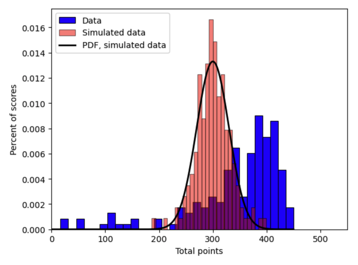
Fig. 19.2 Histograms of one simulation of 161 Econ 381 test scores (2011-2012) from arbitrary truncated normal distribution compared to data#
From that simulation, we can calculate moments from the simulated data just like we did from the actual data. The following function data_moments2() computes the mean and the variance of the simulated data \(x\), where \(x\) is an \(N\times S\) matrix of \(S\) simulations of \(N\) observations each.
def data_moments2(xvals):
    '''
    --------------------------------------------------------------------
    This function computes the two data moments for SMM
    (mean(data), variance(data)) from both the actual data and from the
    simulated data.
    --------------------------------------------------------------------
    INPUTS:
    xvals = (N, S) matrix or (N,) vector, or scalar in (cut_lb, cut_ub),
            test scores data, either real world or simulated. Real world
            data will come in the form (N,). Simulated data comes in the
            form (N,) or (N, S).

    OTHER FUNCTIONS AND FILES CALLED BY THIS FUNCTION: None

    OBJECTS CREATED WITHIN FUNCTION:
    mean_data = scalar or (S,) vector, mean value of test scores data
    var_data  = scalar > 0 or (S,) vector, variance of test scores data

    FILES CREATED BY THIS FUNCTION: None

    RETURNS: mean_data, var_data
    --------------------------------------------------------------------
    '''
    if xvals.ndim == 1:
        mean_data = xvals.mean()
        var_data = xvals.var()
    elif xvals.ndim == 2:
        mean_data = xvals.mean(axis=0)
        var_data = xvals.var(axis=0)

    return mean_data, var_data
mean_data, var_data = data_moments2(data)
print('Data mean =', mean_data)
print('Data variance =', var_data)
mean_sim, var_sim = data_moments2(draws_1)
print('Sim. mean =', mean_sim)
print('Sim. variance =', var_sim)
Data mean = 341.90869565217395
Data variance = 7827.997292398056
Sim. mean = 300.17445658136046
Sim. variance = 1000.626705029347
We can also simulate many \((S)\) data sets of test scores, each with \(N=161\) test scores. The estimate of the model moments will be the average of the simulated data moments across the simulations.
N = 161
S = 100
mu_2 = 300.0
sig_2 = 30.0
cut_lb = 0.0
cut_ub = 450.0
np.random.seed(25)  # Set the random number seed to get same answers every time
unif_vals_2 = sts.uniform.rvs(0, 1, size=(N, S))
draws_2 = trunc_norm_draws(unif_vals_2, mu_2, sig_2,
                           cut_lb, cut_ub)

mean_sim, var_sim = data_moments2(draws_2)
print("Mean test score in each simulation:")
print(mean_sim)
print("")
print("Variance of test scores in each simulation:")
print(var_sim)
mean_mod = mean_sim.mean()
var_mod = var_sim.mean()
print("")
print('Estimated model mean (avg. of means) =', mean_mod)
print('Estimated model variance (avg. of variances) =', var_mod)
Mean test score in each simulation:
[299.17667999 298.61052796 304.45608507 301.37072845 299.66868577
 303.44257561 298.68174796 297.94014672 297.47566228 299.63490045
 298.57207266 299.13235013 296.63826526 300.44460537 302.98678012
 301.09166082 302.89663118 301.50056988 299.56091107 301.94919604
 296.58486163 300.109284   303.35295389 300.4763979  298.52345697
 299.37526236 298.54462388 301.20756546 301.23182905 297.92082255
 302.0881712  300.37792528 302.69523093 298.92838232 296.03376169
 299.9335839  302.69026345 302.0934371  299.70288418 300.88610536
 304.86283252 299.10407269 303.11654222 302.07027394 299.29923542
 298.74552083 297.79965311 301.59852312 300.15616963 301.59864217
 295.52781074 303.98090953 300.31248226 301.44867717 297.78114307
 302.64825256 303.68061798 300.12495043 299.80104697 305.78334207
 300.95811329 297.94097772 303.02458302 300.24287686 305.55084554
 296.62551538 301.73820461 303.91841652 305.97485316 300.25235036
 298.6490962  299.80907094 301.66541992 298.66699545 298.68524191
 301.45696273 301.27407424 298.22269311 301.22887168 299.54314562
 299.85171183 299.26405411 298.87330671 301.59708796 298.46696222
 299.01431864 299.27736899 299.20186117 297.60298908 299.34134778
 296.56023236 300.36842728 299.81705203 300.234357   296.93063956
 301.60442391 299.68503428 298.32917874 300.93011523 298.78807296]

Variance of test scores in each simulation:
[ 854.27400514  793.0403989   841.76252205  819.86183015 1055.80239074
  834.52746835  955.01586149 1033.93476802  804.86989439  715.96784403
  927.66459495  594.40100934  974.32315671  903.2658217   877.78145497
  900.13017505  871.56069402  835.1365732   849.46651395  835.02582303
  939.66718613  654.80578245  998.41113837  815.81618606 1002.68353273
  907.56790563  724.85910396  813.70435378 1015.31786118  975.59759144
  888.63526849  881.81187368  842.94152651  976.74617301  978.23045295
  790.85144559  933.04687473  987.37433204  980.14458376 1003.34539581
  859.63957381 1050.9870203   901.66724764  967.15290016 1133.2532708
 1033.60468078  810.90856957  930.53152973  921.0020767   802.31271115
  928.68723732 1046.31773806  932.0434472  1025.05965686  951.23678849
  839.58583279  941.39252702  751.71431141  841.4610679  1021.10990195
  863.80405021  849.16404517  819.12655726 1095.10022731  848.76703098
  797.43467707  823.16623979 1056.73087072  821.12496192  917.86308975
  841.00526807  862.52415389  937.44315325  884.41413606  933.28154226
  864.67286651  992.96039373  856.4044805   868.37693837  954.32843377
  814.35548352  758.33184649  861.16008799  917.8168036   980.31470517
  821.32422902 1057.5979759   843.6883495   941.15291878  925.33449079
  778.30674576  856.47550771  920.80553617  902.19187292  918.9232
  880.47284712  841.07711245  925.82668059 1037.04590733  925.75216207]

Estimated model mean (avg. of means) = 300.28595134427394
Estimated model variance (avg. of variances) = 898.7468703753616
Our SMM model moments \(\hat{m}(\tilde{scores}_i|\mu,\sigma)\) are an estimate of the true models moments that we got in the GMM case by integrating using the PDF of the truncated normal distribution. Our SMM moments we got by simulating the data \(S\) times and taking the average of the simulated data moments across the simulations as our estimator of the model moments.
Define the error vector as the vector of percent deviations of the model moments from the data moments.
The SMM estimator for this moment vector is the following.
Now let’s define a criterion function that takes as inputs the parameters and the estimator for the weighting matrix \(\hat{W}\).
def err_vec2(data_vals, unif_vals, mu, sigma, cut_lb, cut_ub, simple):
    '''
    --------------------------------------------------------------------
    This function computes the vector of moment errors (in percent
    deviation from the data moment vector) for SMM.
    --------------------------------------------------------------------
    INPUTS:
    data_vals = (N,) vector, test scores data
    unif_vals = (N, S) matrix, S simulations of N observations from
                uniform distribution U(0,1)
    mu        = scalar, mean of the nontruncated normal distribution
                from which the truncated normal is derived
    sigma     = scalar > 0, standard deviation of the nontruncated
                normal distribution from which the truncated normal is
                derived
    cut_lb    = scalar or string, ='None' if no lower bound cutoff is
                given, otherwise is scalar lower bound value of
                distribution. Values below this cutoff have zero
                probability
    cut_ub    = scalar or string, ='None' if no upper bound cutoff is
                given, otherwise is scalar lower bound value of
                distribution. Values below this cutoff have zero
                probability
    simple    = boolean, =True if errors are simple difference, =False
                if errors are percent deviation from data moments

    OTHER FUNCTIONS AND FILES CALLED BY THIS FUNCTION:
        trunc_norm_draws()
        data_moments()

    OBJECTS CREATED WITHIN FUNCTION:
    mean_data  = scalar, mean value of data
    var_data   = scalar > 0, variance of data
    moms_data  = (2, 1) matrix, column vector of two data moments
    mean_model = scalar, estimated mean value from model
    var_model  = scalar > 0, estimated variance from model
    moms_model = (2, 1) matrix, column vector of two model moments
    err_vec    = (2, 1) matrix, column vector of two moment error
                 functions

    FILES CREATED BY THIS FUNCTION: None

    RETURNS: err_vec
    --------------------------------------------------------------------
    '''
    sim_vals = trunc_norm_draws(unif_vals, mu, sigma, cut_lb, cut_ub)
    mean_data, var_data = data_moments2(data_vals)
    moms_data = np.array([[mean_data], [var_data]])
    mean_sim, var_sim = data_moments2(sim_vals)
    mean_model = mean_sim.mean()
    var_model = var_sim.mean()
    moms_model = np.array([[mean_model], [var_model]])
    if simple:
        err_vec = moms_model - moms_data
    else:
        err_vec = (moms_model - moms_data) / moms_data

    return err_vec


def criterion(params, *args):
    '''
    --------------------------------------------------------------------
    This function computes the SMM weighted sum of squared moment errors
    criterion function value given parameter values and an estimate of
    the weighting matrix.
    --------------------------------------------------------------------
    INPUTS:
    params    = (2,) vector, ([mu, sigma])
    mu        = scalar, mean of the normally distributed random variable
    sigma     = scalar > 0, standard deviation of the normally
                distributed random variable
    args      = length 6 tuple,
                (xvals, unif_vals, cut_lb, cut_ub, W_hat, simple)
    xvals     = (N,) vector, values of the truncated normally
                distributed random variable
    unif_vals = (N, S) matrix, matrix of draws from U(0,1) distribution.
                This fixes the seed of the draws for the simulations
    cut_lb    = scalar or string, ='None' if no lower bound cutoff is
                given, otherwise is scalar lower bound value of
                distribution. Values below this cutoff have zero
                probability
    cut_ub    = scalar or string, ='None' if no upper bound cutoff is
                given, otherwise is scalar lower bound value of
                distribution. Values below this cutoff have zero
                probability
    W_hat     = (R, R) matrix, estimate of optimal weighting matrix
    simple    = Boolean, =True if error vec is simple difference,
                =False if error vec is percent difference

    OTHER FUNCTIONS AND FILES CALLED BY THIS FUNCTION:
        err_vec2()

    OBJECTS CREATED WITHIN FUNCTION:
    err        = (2, 1) matrix, column vector of two moment error
                 functions
    crit_val   = scalar > 0, GMM criterion function value

    FILES CREATED BY THIS FUNCTION: None

    RETURNS: crit_val
    --------------------------------------------------------------------
    '''
    mu, sigma = params
    xvals, unif_vals, cut_lb, cut_ub, W_hat, simple = args
    err = err_vec2(xvals, unif_vals, mu, sigma, cut_lb, cut_ub,
                   simple)
    crit_val = err.T @ W_hat @ err

    return crit_val
mu_test = 400
sig_test = 70
cut_lb = 0.0
cut_ub = 450.0
sim_vals = trunc_norm_draws(unif_vals_2, mu_test, sig_test, cut_lb, cut_ub)
mean_sim, var_sim = data_moments2(sim_vals)
mean_mod = mean_sim.mean()
var_mod = var_sim.mean()
err_vec2(data, unif_vals_2, mu_test, sig_test, cut_lb, cut_ub, simple=False)
crit_test = criterion(np.array([mu_test, sig_test]), data, unif_vals_2,
                      0.0, 450.0, np.eye(2), False)
print("Average of mean test scores across simulations is:", mean_mod)
print("")
print("Average variance of test scores across simulations is:", var_mod)
print("")
print("Criterion function value is:", crit_test[0][0])
Average of mean test scores across simulations is: 372.0777280048037

Average variance of test scores across simulations is: 2663.8708280174988

Criterion function value is: 0.4429893115777857
Now we can perform the SMM estimation using SciPy’s minimize function to choose the values of \(\mu\) and \(\sigma\) of the truncated normal distribution that best fit the data by minimizing the crietrion function. Let’s start with the identity matrix as our estimate for the optimal weighting matrix \(W = I\).
mu_init_1 = 300
sig_init_1 = 30
params_init_1 = np.array([mu_init_1, sig_init_1])
W_hat1_1 = np.eye(2)
smm_args1_1 = (data, unif_vals_2, cut_lb, cut_ub, W_hat1_1, False)
results1_1 = opt.minimize(criterion, params_init_1, args=(smm_args1_1),
                          method='L-BFGS-B',
                          bounds=((1e-10, None), (1e-10, None)))
mu_SMM1_1, sig_SMM1_1 = results1_1.x
print('mu_SMM1_1=', mu_SMM1_1, ' sig_SMM1_1=', sig_SMM1_1)
mu_SMM1_1= 612.3371352249138 sig_SMM1_1= 197.26434895262162
mean_data, var_data = data_moments2(data)
print('Data mean of scores =', mean_data, ', Data variance of scores =', var_data)
sim_vals_1 = trunc_norm_draws(unif_vals_2, mu_SMM1_1, sig_SMM1_1, cut_lb, cut_ub)
mean_sim_1, var_sim_1 = data_moments2(sim_vals_1)
mean_model_1 = mean_sim_1.mean()
var_model_1 = var_sim_1.mean()
err_1 = err_vec2(data, unif_vals_2, mu_SMM1_1, sig_SMM1_1, cut_lb, cut_ub,
                 False).reshape(2,)
print("")
print('Model mean 1 =', mean_model_1, ', Model variance 1 =', var_model_1)
print("")
print('Error vector 1 =', err_1)
print("")
print("Results from scipy.opmtimize.minimize:")
print(results1_1)
Data mean of scores = 341.90869565217395 , Data variance of scores = 7827.997292398056

Model mean 1 = 341.6692110494425 , Model variance 1 = 7827.864496338213

Error vector 1 = [-7.00434373e-04 -1.69642445e-05]

Results from scipy.opmtimize.minimize:
  message: CONVERGENCE: NORM_OF_PROJECTED_GRADIENT_<=_PGTOL
  success: True
   status: 0
      fun: 4.908960959342433e-07
        x: [ 6.123e+02  1.973e+02]
      nit: 17
      jac: [-7.436e-07  2.350e-06]
     nfev: 72
     njev: 24
 hess_inv: <2x2 LbfgsInvHessProduct with dtype=float64>
Let’s plot the PDF implied by these SMM estimates \((\hat{\mu}_{SMM},\hat{\sigma}_{SMM})=(612.337, 197.264)\) against the histogram of the data in Figure 19.3 below.
# Plot the histogram of the data
count, bins, ignored = plt.hist(data, 30, density=True,
                                edgecolor='black', linewidth=1.2, label='data')
plt.title('Econ 381 scores: 2011-2012', fontsize=20)
plt.xlabel('Total points')
plt.ylabel('Percent of scores')
plt.xlim([0, 550])  # This gives the xmin and xmax to be plotted"

# Plot the estimated SMM PDF
dist_pts = np.linspace(0, 450, 500)
plt.plot(dist_pts, trunc_norm_pdf(dist_pts, mu_SMM1_1, sig_SMM1_1, 0.0, 450.0),
         linewidth=2, color='k', label='PDF: ($\hat{\mu}_{SMM1}$,$\hat{\sigma}_{SMM1}$)=(612.34, 197.26)')
plt.legend(loc='upper left')

plt.show()

Fig. 19.3 SMM-estimated PDF function and data histogram, 2 moments, identity weighting matrix, Econ 381 scores (2011-2012)#
That looks just like the maximum likelihood estimate from the Maximum Likelihood Estimation chapter. Figure 19.4 below shows what the minimizer is doing. The figure shows the criterion function surface for different of \(\mu\) and \(\sigma\) in the truncated normal distribution. The minimizer is searching for the parameter values that give the lowest criterion function value.
mu_vals = np.linspace(60, 700, 90)
sig_vals = np.linspace(20, 250, 100)
crit_vals = np.zeros((90, 100))
crit_args = (data, unif_vals_2, cut_lb, cut_ub, W_hat1_1, False)
for mu_ind in range(90):
    for sig_ind in range(100):
        crit_params = np.array([mu_vals[mu_ind], sig_vals[sig_ind]])
        crit_vals[mu_ind, sig_ind] = criterion(crit_params, *crit_args)[0][0]

mu_mesh, sig_mesh = np.meshgrid(mu_vals, sig_vals)

crit_SMM1_1 = criterion(np.array([mu_SMM1_1, sig_SMM1_1]), *crit_args)[0][0]

fig, ax = plt.subplots(subplot_kw={"projection": "3d"})
ax.plot_surface(mu_mesh.T, sig_mesh.T, crit_vals, rstride=8,
                cstride=1, cmap=cmap1, alpha=0.9)
ax.scatter(mu_SMM1_1, sig_SMM1_1, crit_SMM1_1, color='red', marker='o',
           s=18, label='SMM1 estimate')
ax.view_init(elev=12, azim=30, roll=0)
ax.set_title('Criterion function for values of mu and sigma')
ax.set_xlabel(r'$\mu$')
ax.set_ylabel(r'$\sigma$')
ax.set_zlabel(r'Crit. func.')
plt.tight_layout()

plt.show()

Fig. 19.4 Criterion function surface for values of \(\mu\) and \(\sigma\) for SMM estimation of truncated normal with two moments and identity weighting matrix (SMM estimate shown as red dot)#
Let’s compute the SMM estimator for the variance-covariance matrix \(\hat{\Sigma}_{SMM}\) of our SMM estimates \(\hat{\theta}_{SMM}\) using the equation in Section Variance-Covariance Estimator of \hat{\theta} based on the Jacobian \(d(\tilde{x},x|\hat{\theta}_{SMM})\) of the moment error vector \(e(\tilde{x},x|\hat{\theta}_{SMM})\) from the criterion function at the estimated (optimal) parameter values \(\hat{\theta}_{SMM}\). We first write a function that computes the Jacobian matrix \(d(x|\hat{\theta}_{SMM})\), which has shape \(2\times 2\) in this case with two moments \(R=2\).
def Jac_err2(data_vals, unif_vals, mu, sigma, cut_lb, cut_ub, simple=False):
    '''
    This function computes the Jacobian matrix of partial derivatives of the
    R x 1 moment error vector e(x|theta) with respect to the K parameters
    theta_i in the K x 1 parameter vector theta. The resulting matrix is R x K
    Jacobian.
    '''
    Jac_err = np.zeros((2, 2))
    h_mu = 1e-4 * mu
    h_sig = 1e-4 * sigma
    Jac_err[:, 0] = (
        (err_vec2(xvals, unif_vals, mu + h_mu, sigma, cut_lb, cut_ub, simple) -
         err_vec2(xvals, unif_vals, mu - h_mu, sigma, cut_lb, cut_ub, simple)) /
        (2 * h_mu)
    ).flatten()
    Jac_err[:, 1] = (
        (err_vec2(xvals, unif_vals, mu, sigma + h_sig, cut_lb, cut_ub, simple) -
         err_vec2(xvals, unif_vals, mu, sigma - h_sig, cut_lb, cut_ub, simple)) /
        (2 * h_sig)
    ).flatten()

    return Jac_err
S = unif_vals_2.shape[1]
d_err2 = Jac_err2(data, unif_vals_2, mu_SMM1_1, sig_SMM1_1, 0.0, 450.0, False)
print("Jacobian matrix of derivatives of moment error functions is:")
print(d_err2)
print("")
print("Weighting matrix W is:")
print(W_hat1_1)
SigHat2 = (1 / S) * lin.inv(d_err2.T @ W_hat1_1 @ d_err2)
print("")
print("Variance-covariance matrix of estimated parameter vector is:")
print(SigHat2)
print("")
print('Std. err. mu_hat=', np.sqrt(SigHat2[0, 0]))
print('Std. err. sig_hat=', np.sqrt(SigHat2[1, 1]))
Jacobian matrix of derivatives of moment error functions is:
[[ 0.00089749 -0.00290433]
 [-0.00114132  0.00445698]]

Weighting matrix W is:
[[1. 0.]
 [0. 1.]]

Variance-covariance matrix of estimated parameter vector is:
[[602535.18442996 163802.17330123]
 [163802.17330123  44883.79092131]]

Std. err. mu_hat= 776.23139876583
Std. err. sig_hat= 211.85794986573154
This SMM estimation methodology of estimating \(\mu\) and \(\sigma\) from the truncated normal distribution to fit the distribution of Econ 381 test scores using two moments from the data and using the identity matrix as the optimal weighting matrix is not very precise. The standard errors for the estimates of \(\hat{mu}\) and \(\hat{sigma}\) are bigger than their values.
In the next section, we see if we can get more accurate estimates (lower criterion function values) of \(\hat{mu}\) and \(\hat{sigma}\) with more precise standard errors by using the two-step optimal weighting matrix described in Section Two-step variance-covariance estimator of W.
19.4.1.2. Two moments, two-step optimal weighting matrix#
Similar to the maximum likelihood estimation problem in Chapter Maximum Likelihood Estimation, it looks like the minimum value of the criterion function shown in Figure 19.4 is roughly equal for a specific portion increase of \(\mu\) and \(\sigma\) together. That is, the estimation problem with these two moments probably has a correspondence of values of \(\mu\) and \(\sigma\) that give roughly the same minimum criterion function value. This issue has two possible solutions.
Maybe we need the two-step variance covariance estimator to calculate a “more” optimal weighting matrix \(W\).
Maybe our two moments aren’t very good moments for fitting the data.
Let’s first try the two-step weighting matrix.
def get_Err_mat2(pts, unif_vals, mu, sigma, cut_lb, cut_ub, simple=False):
    '''
    --------------------------------------------------------------------
    This function computes the R x S matrix of errors from each
    simulated moment for each moment error. In this function, we have
    hard coded R = 2.
    --------------------------------------------------------------------
    INPUTS:
    xvals     = (N,) vector, test scores data
    unif_vals = (N, S) matrix, uniform random variables that generate
                the N observations of simulated data for S simulations
    mu        = scalar, mean of the normally distributed random variable
    sigma     = scalar > 0, standard deviation of the normally
                distributed random variable
    cut_lb    = scalar or string, ='None' if no cutoff is given,
                otherwise is scalar lower bound value of distribution.
                Values below this value have zero probability
    cut_ub    = scalar or string, ='None' if no cutoff is given,
                otherwise is scalar upper bound value of distribution.
                Values above this value have zero probability
    simple    = boolean, =True if errors are simple difference, =False
                if errors are percent deviation from data moments

    OTHER FUNCTIONS AND FILES CALLED BY THIS FUNCTION:
        model_moments()

    OBJECTS CREATED WITHIN FUNCTION:
    R          = integer = 2, hard coded number of moments
    S          = integer >= R, number of simulated datasets
    Err_mat    = (R, S) matrix, error by moment and simulated data
    mean_model = scalar, mean value from model
    var_model  = scalar > 0, variance from model

    FILES CREATED BY THIS FUNCTION: None

    RETURNS: Err_mat
    --------------------------------------------------------------------
    '''
    R = 2
    S = unif_vals.shape[1]
    Err_mat = np.zeros((R, S))
    mean_data, var_data = data_moments2(pts)
    sim_vals = trunc_norm_draws(unif_vals, mu, sigma, cut_lb, cut_ub)
    mean_model, var_model = data_moments2(sim_vals)
    if simple:
        Err_mat[0, :] = mean_model - mean_data
        Err_mat[1, :] = var_model - var_data
    else:
        Err_mat[0, :] = (mean_model - mean_data) / mean_data
        Err_mat[1, :] = (var_model - var_data) / var_data

    return Err_mat
Err_mat2 = get_Err_mat2(data, unif_vals_2, mu_SMM1_1, sig_SMM1_1, 0.0, 450.0, False)
VCV2 = (1 / unif_vals_2.shape[1]) * (Err_mat2 @ Err_mat2.T)
print("2nd stage est. of var-cov matrix of moment error vec across sims:")
print(VCV2)
W_hat2_1 = lin.inv(VCV2)
print("")
print("2nd state est. of optimal weighting matrix:")
print(W_hat2_1)
2nd stage est. of var-cov matrix of moment error vec across sims:
[[ 0.00033411 -0.00142289]
 [-0.00142289  0.01592879]]

2nd state est. of optimal weighting matrix:
[[4830.88530228  431.53378728]
 [ 431.53378728  101.32749623]]
params_init2_1 = np.array([mu_SMM1_1, sig_SMM1_1])
smm_args2_1 = (data, unif_vals_2, cut_lb, cut_ub, W_hat2_1, False)
results2_1 = opt.minimize(criterion, params_init2_1, args=(smm_args2_1),
                         method='L-BFGS-B',
                         bounds=((1e-10, None), (1e-10, None)))
mu_SMM2_1, sig_SMM2_1 = results2_1.x
print('mu_SMM2_1=', mu_SMM2_1, ' sig_SMM2_1=', sig_SMM2_1)
mu_SMM2_1= 619.4303074248937 sig_SMM2_1= 199.0747813692372
Look at how much smaller (more efficient) the estimated standard errors are in this case with the two-step optimal weighting matrix \(\hat{W}_{2step}\).
d_err2_2 = Jac_err2(data, unif_vals_2, mu_SMM2_1, sig_SMM2_1, 0.0, 450.0, False)
print("Jacobian matrix of derivatives of moment error functions is:")
print(d_err2_2)
print("")
print("Weighting matrix W is:")
print(W_hat2_1)
SigHat2_2 = (1 / S) * lin.inv(d_err2_2.T @ W_hat2_1 @ d_err2_2)
print("")
print("Variance-covariance matrix of estimated parameter vector is:")
print(SigHat2_2)
print("")
print('Std. err. mu_hat=', np.sqrt(SigHat2_2[0, 0]))
print('Std. err. sig_hat=', np.sqrt(SigHat2_2[1, 1]))
Jacobian matrix of derivatives of moment error functions is:
[[ 0.00088129 -0.00288863]
 [-0.0011259   0.00443426]]

Weighting matrix W is:
[[4830.88530228  431.53378728]
 [ 431.53378728  101.32749623]]

Variance-covariance matrix of estimated parameter vector is:
[[2397.38054356  745.29670501]
 [ 745.29670501  232.01757158]]

Std. err. mu_hat= 48.963052841479445
Std. err. sig_hat= 15.232123016118733
19.4.1.3. Four moments, identity matrix weighting matrix#
Using a better weighting matrix didn’t improve our estimates or fit very much—the estimates of \(\hat{mu}\) and \(\hat{\sigma}\) and the corresponding minimum criterion function value. But it did improve our standard errors. But even with the optimal weighting matrix, our standard errors still look pretty big. This might mean that we did not choose good moments for fitting the data. Let’s try some different moments. How about four moments to match.
The percent of observations greater than 430 (between 430 and 450)
The percent of observations between 320 and 430
The percent of observations between 220 and 320
The percent of observations less than 220 (between 0 and 220)
This means we are using four moments \(R=4\) to identify two paramters \(\mu\) and \(\sigma\) (\(K=2\)). This problem is now overidentified (\(R>K\)). This is often a desired approach for SMM estimation.
def data_moments4(xvals):
    '''
    --------------------------------------------------------------------
    This function computes the four data moments for SMM
    (binpct_1, binpct_2, binpct_3, binpct_4) from both the actual data
    and from the simulated data.
    --------------------------------------------------------------------
    INPUTS:
    xvals = (N, S) matrix, (N,) vector, or scalar in (cut_lb, cut_ub),
            test scores data, either real world or simulated. Real world
            data will come in the form (N,). Simulated data comes in the
            form (N,) or (N, S).

    OTHER FUNCTIONS AND FILES CALLED BY THIS FUNCTION: None

    OBJECTS CREATED WITHIN FUNCTION:
    bpct_1 = scalar in [0, 1] or (S,) vector, percent of observations
             0 <= x < 220
    bpct_2 = scalar in [0, 1] or (S,) vector, percent of observations
             220 <= x < 320
    bpct_3 = scalar in [0, 1] or (S,) vector, percent of observations
             320 <= x < 430
    bpct_4 = scalar in [0, 1] or (S,) vector, percent of observations
             430 <= x <= 450

    FILES CREATED BY THIS FUNCTION: None

    RETURNS: bpct_1, bpct_2, bpct_3, bpct_4
    --------------------------------------------------------------------
    '''
    if xvals.ndim == 1:
        bpct_1 = (xvals < 220).sum() / xvals.shape[0]
        bpct_2 = ((xvals >=220) & (xvals < 320)).sum() / xvals.shape[0]
        bpct_3 = ((xvals >=320) & (xvals < 430)).sum() / xvals.shape[0]
        bpct_4 = (xvals >= 430).sum() / xvals.shape[0]
    if xvals.ndim == 2:
        bpct_1 = (xvals < 220).sum(axis=0) / xvals.shape[0]
        bpct_2 = (((xvals >=220) & (xvals < 320)).sum(axis=0) /
                    xvals.shape[0])
        bpct_3 = (((xvals >=320) & (xvals < 430)).sum(axis=0) /
                    xvals.shape[0])
        bpct_4 = (xvals >= 430).sum(axis=0) / xvals.shape[0]

    return bpct_1, bpct_2, bpct_3, bpct_4
def err_vec4(data_vals, unif_vals, mu, sigma, cut_lb, cut_ub, simple):
    '''
    --------------------------------------------------------------------
    This function computes the vector of moment errors (in percent
    deviation from the data moment vector) for SMM.
    --------------------------------------------------------------------
    INPUTS:
    data_vals = (N,) vector, test scores data
    unif_vals = (N, S) matrix, uniform values that generate S
                simulations of N observations
    mu        = scalar, mean of the nontruncated normal distribution
                from which the truncated normal is derived
    sigma     = scalar > 0, standard deviation of the nontruncated
                normal distribution from which the truncated normal is
                derived
    cut_lb    = scalar or string, ='None' if no lower bound cutoff is
                given, otherwise is scalar lower bound value of
                distribution. Values below this cutoff have zero
                probability
    cut_ub    = scalar or string, ='None' if no upper bound cutoff is
                given, otherwise is scalar lower bound value of
                distribution. Values below this cutoff have zero
                probability
    simple    = boolean, =True if errors are simple difference, =False
                if errors are percent deviation from data moments

    OTHER FUNCTIONS AND FILES CALLED BY THIS FUNCTION:
        data_moments4()

    OBJECTS CREATED WITHIN FUNCTION:
    mean_data  = scalar, mean value of data
    var_data   = scalar > 0, variance of data
    moms_data  = (4, 1) matrix, column vector of two data moments
    mean_model = scalar, mean value from model
    var_model  = scalar > 0, variance from model
    moms_model = (2, 1) matrix, column vector of two model moments
    err_vec    = (2, 1) matrix, column vector of two moment error
                 functions

    FILES CREATED BY THIS FUNCTION: None

    RETURNS: err_vec
    --------------------------------------------------------------------
    '''
    sim_vals = trunc_norm_draws(unif_vals, mu, sigma, cut_lb, cut_ub)
    bpct_1_dat, bpct_2_dat, bpct_3_dat, bpct_4_dat = \
        data_moments4(data_vals)
    moms_data = np.array([[bpct_1_dat], [bpct_2_dat], [bpct_3_dat],
                          [bpct_4_dat]])
    bpct_1_sim, bpct_2_sim, bpct_3_sim, bpct_4_sim = \
        data_moments4(sim_vals)
    bpct_1_mod = bpct_1_sim.mean()
    bpct_2_mod = bpct_2_sim.mean()
    bpct_3_mod = bpct_3_sim.mean()
    bpct_4_mod = bpct_4_sim.mean()
    moms_model = np.array([[bpct_1_mod], [bpct_2_mod], [bpct_3_mod],
                          [bpct_4_mod]])
    if simple:
        err_vec = moms_model - moms_data
    else:
        err_vec = (moms_model - moms_data) / moms_data

    return err_vec
def criterion4(params, *args):
    '''
    --------------------------------------------------------------------
    This function computes the SMM weighted sum of squared moment errors
    criterion function value given parameter values and an estimate of
    the weighting matrix.
    --------------------------------------------------------------------
    INPUTS:
    params    = (2,) vector, ([mu, sigma])
    mu        = scalar, mean of the normally distributed random variable
    sigma     = scalar > 0, standard deviation of the normally
                distributed random variable
    args      = length 5 tuple,
                (xvals, unif_vals, cut_lb, cut_ub, W_hat)
    xvals     = (N,) vector, values of the truncated normally
                distributed random variable
    unif_vals = (N, S) matrix, matrix of draws from U(0,1) distribution.
                This fixes the seed of the draws for the simulations
    cut_lb    = scalar or string, ='None' if no lower bound cutoff is
                given, otherwise is scalar lower bound value of
                distribution. Values below this cutoff have zero
                probability
    cut_ub    = scalar or string, ='None' if no upper bound cutoff is
                given, otherwise is scalar lower bound value of
                distribution. Values below this cutoff have zero
                probability
    W_hat     = (R, R) matrix, estimate of optimal weighting matrix

    OTHER FUNCTIONS AND FILES CALLED BY THIS FUNCTION:
        norm_pdf()

    OBJECTS CREATED WITHIN FUNCTION:
    err        = (2, 1) matrix, column vector of two moment error
                 functions
    crit_val   = scalar > 0, GMM criterion function value

    FILES CREATED BY THIS FUNCTION: None

    RETURNS: crit_val
    --------------------------------------------------------------------
    '''
    mu, sigma = params
    xvals, unif_vals, cut_lb, cut_ub, W_hat = args

    # # These next two lines diagnose a problems in the next frame
    # print('mu=', mu)
    # print('sigma', sigma)

    err = err_vec4(xvals, unif_vals, mu, sigma, cut_lb, cut_ub,
                   simple=False)
    crit_val = err.T @ W_hat @ err

    return crit_val
Now we will execute the SMM minimization problem, but a strange issue will arise. And the issue has to do with the minimizer.
mu_init4_1 = 300
sig_init4_1 = 30
params_init4_1 = np.array([mu_init4_1, sig_init4_1])
W_hat4_1 = np.eye(4)
smm_args4_1 = (data, unif_vals_2, 0.0, 450, W_hat4_1)
results4_1 = opt.minimize(criterion4, params_init4_1, args=(smm_args4_1),
                          method='L-BFGS-B',
                          bounds=((1e-10, None), (1e-10, None)))
mu_SMM4_1, sig_SMM4_1 = results4_1.x
print('mu_SMM4_1=', mu_SMM4_1, ' sig_SMM4_1', sig_SMM4_1)
print(results4_1)
mu_SMM4_1= 300.0  sig_SMM4_1 30.0
  message: CONVERGENCE: NORM_OF_PROJECTED_GRADIENT_<=_PGTOL
  success: True
   status: 0
      fun: 12.836206045344852
        x: [ 3.000e+02  3.000e+01]
      nit: 0
      jac: [ 0.000e+00  0.000e+00]
     nfev: 3
     njev: 1
 hess_inv: <2x2 LbfgsInvHessProduct with dtype=float64>
Note that the optimization problem only did three function evaluations, and it decided that the parameter values that minimized the criterion function are the initial values. Something is wrong.
To see what is happening in the minimizer, let’s insert a line in the criterion4() function that prints out the values of \(\mu\) and \(\sigma\) for each function evaluation in the minimizer as well as the error vector associated with each guess of \(\mu\) and \(\sigma\).
Note that the three function evaluations are for guesses of \(\mu\) and \(\sigma\) of:
Guess 1: \(\mu\)=
mu_initand \(\sigma\)=sig_initGuess 2: \(\mu\)=
mu_init + 0.00000001and \(\sigma\)=sig_initGuess 3: \(\mu\)=
mu_initand \(\sigma\)=sig_init + 0.00000001
This is the L-BFGS-B method’s way of computing the Jacobian or slope (gradient) matrix of the criterion function by finite difference. However, the epsilon of 0.00000001 seems to be too small. We can set this step size to be bigger by using the minimize() function’s options={} argument.
The options={} argument in the minimize() function is a dictionary of solver options available to each particular method. In our case, we want to look at the options={} arguments for the L-BFGS-B method of the scipy.minimize() function. Looking at this documentation, we find that we can set the eps option to something other than its default which is options={'eps': 1e-08}. In our case, we want to set that epsilon value used the finite differnce estimation of the Jacobian to be something bigger. Our means and variances seem to be in the 100’s, so let’s see if we get a solution setting the epsilon equal to 1.0.
results4_1 = opt.minimize(criterion4, params_init4_1, args=(smm_args4_1),
                          method='L-BFGS-B',
                          bounds=((1e-10, None), (1e-10, None)),
                          options={'eps': 1.0})
mu_SMM4_1, sig_SMM4_1 = results4_1.x
print('mu_SMM4_1=', mu_SMM4_1, ' sig_SMM4_1', sig_SMM4_1)
print(results4_1)
mu_SMM4_1= 362.560593472098  sig_SMM4_1 46.5751519565219
  message: CONVERGENCE: REL_REDUCTION_OF_F_<=_FACTR*EPSMCH
  success: True
   status: 0
      fun: 0.9819514324825378
        x: [ 3.626e+02  4.658e+01]
      nit: 8
      jac: [ 2.845e-03 -1.022e-03]
     nfev: 144
     njev: 48
 hess_inv: <2x2 LbfgsInvHessProduct with dtype=float64>
Figure 19.5 shows the plot the PDF implied by these results \(\hat{\mu}=362.2\) and \(\hat{\sigma}=46.6\) against the histogram of the data.
Show code cell source
# Plot the histogram of the data
count, bins, ignored = plt.hist(
    data, 30, density=True, edgecolor='black', linewidth=1.2, label='Data'
)
plt.xlabel('Total points')
plt.ylabel('Percent of scores')
plt.xlim([0, 550])  # This gives the xmin and xmax to be plotted"

# Plot the estimated SMM PDF
dist_pts = np.linspace(cut_lb, cut_ub, 500)
plt.plot(
    dist_pts, trunc_norm_pdf(dist_pts, mu_SMM4_1, sig_SMM4_1, cut_lb, cut_ub), linewidth=2, color='k', label=(
            f"1: $\mu$={np.round(mu_SMM4_1, decimals=1)}, " +
            f"$\sigma$={np.round(sig_SMM4_1, decimals=1)}")
        )
plt.legend(loc='upper left')

plt.show()
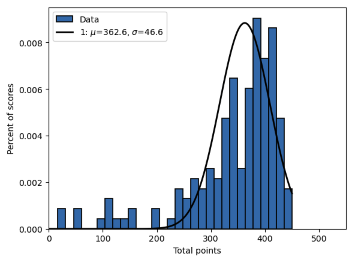
Fig. 19.5 SMM-estimated PDF function and data histogram, 4 moments, identity weighting matrix, Econ 381 scores (2011-2012)#
Let’s print the data moments and the model moments as well as the error vector evaluated at the SMM estimates.
bpct_1_data, bpct_2_data, bpct_3_data, bpct_4_data = data_moments4(data)
print("Data moments =")
print(bpct_1_data, bpct_2_data, bpct_3_data, bpct_4_data)
sim_vals4_1 = trunc_norm_draws(unif_vals_2, mu_SMM4_1, sig_SMM4_1, 0.0, 450)
bpct_1_sim4_1, bpct_2_sim4_1, bpct_3_sim4_1, bpct_4_sim4_1 = \
    data_moments4(sim_vals4_1)
bpct_1_model4_1 = bpct_1_sim4_1.mean()
bpct_2_model4_1 = bpct_2_sim4_1.mean()
bpct_3_model4_1 = bpct_3_sim4_1.mean()
bpct_4_model4_1 = bpct_4_sim4_1.mean()
print("")
print("Model moments =")
print(bpct_1_model4_1, bpct_2_model4_1, bpct_3_model4_1, bpct_4_model4_1)
err4_1 = err_vec4(data, unif_vals_2, mu_SMM4_1, sig_SMM4_1, 0.0, 450, False)
crit_params = np.array([mu_SMM4_1, sig_SMM4_1])
criterion4_1 = criterion4(crit_params, data, unif_vals_2, 0.0, 450, W_hat4_1)
print("")
print('Error vector (pct. dev.) =', err4_1.reshape(4,))
print("")
print('Criterion func val=', criterion4_1[0][0])
Data moments =
0.08695652173913043 0.17391304347826086 0.6894409937888198 0.049689440993788817

Model moments =
0.0017391304347826085 0.1820496894409938 0.7702484472049688 0.04596273291925465

Error vector (pct. dev.) = [-0.98        0.04678571  0.11720721 -0.075     ]

Criterion func val= 0.9819514324825378
We can compute the estimator of the variance-covariance matrix \(\hat{\Sigma}\) of the SMM parameter estimator by computing the Jacobian of the error vector. In this case, the Jacobian \(d(\tilde{x},x|\theta)\) is \(R\times K = 4\times 2\).
def Jac_err4(data_vals, unif_vals, mu, sigma, cut_lb, cut_ub, simple=False):
    '''
    This function computes the Jacobian matrix of partial derivatives of the R x 1 moment
    error vector e(x|theta) with respect to the K parameters theta_i in the K x 1 parameter vector
    theta. The resulting matrix is R x K Jacobian.
    '''
    Jac_err = np.zeros((4, 2))
    h_mu = 1e-4 * mu
    h_sig = 1e-4 * sigma
    Jac_err[:, 0] = \
        ((err_vec4(data_vals, unif_vals, mu + h_mu, sigma, cut_lb, cut_ub, simple) -
          err_vec4(data_vals, unif_vals, mu - h_mu, sigma, cut_lb, cut_ub, simple)) / (2 * h_mu)).flatten()
    Jac_err[:, 1] = \
        ((err_vec4(data_vals, unif_vals, mu, sigma + h_sig, cut_lb, cut_ub, simple) -
          err_vec4(data_vals, unif_vals, mu, sigma - h_sig, cut_lb, cut_ub, simple)) / (2 * h_sig)).flatten()

    return Jac_err
d_err4_1 = Jac_err4(data, unif_vals_2, mu_SMM4_1, sig_SMM4_1, 0.0, 450.0, False)
print("Jacobian matrix of derivatives of moment error functions (4 x 2) is:")
print(d_err4_1)
print("")
print("Estimate of optimal weighting matrix is identity matrix (4 x 4):")
print(W_hat4_1)
SigHat4_1 = (1 / S) * lin.inv(d_err4_1.T @ W_hat4_1 @ d_err4_1)
print("")
print("Variance-covariance matrix of estimated parameter vector is:")
print(SigHat4_1)
print("")
print('Std. err. mu_hat=', np.sqrt(SigHat4_1[0, 0]))
print('Std. err. sig_hat=', np.sqrt(SigHat4_1[1, 1]))
Jacobian matrix of derivatives of moment error functions (4 x 2) is:
[[ 0.          0.        ]
 [-0.05417814  0.07668099]
 [ 0.01242414 -0.01934295]
 [ 0.0172385   0.        ]]

Estimate of optimal weighting matrix is identity matrix (4 x 4):
[[1. 0. 0. 0.]
 [0. 1. 0. 0.]
 [0. 0. 1. 0.]
 [0. 0. 0. 1.]]

Variance-covariance matrix of estimated parameter vector is:
[[33.48770545 23.53170341]
 [23.53170341 18.13459776]]

Std. err. mu_hat= 5.786856266717126
Std. err. sig_hat= 4.258473642422245
19.4.1.4. Four moments, two-step optimal weighting matrix#
Let’s see how much things change if we use the two-step estimator for the optimal weighting matrix \(W\) instead of the identity matrix.
def get_Err_mat4(data, unif_vals, mu, sigma, cut_lb, cut_ub, simple=False):
    '''
    --------------------------------------------------------------------
    This function computes the R x S matrix of errors from each
    simulated moment for each moment error. In this function, we have
    hard coded R = 4.
    --------------------------------------------------------------------
    INPUTS:
    xvals     = (N,) vector, test scores data
    unif_vals = (N, S) matrix, uniform random variables that generate
                the N observations of simulated data for S simulations
    mu        = scalar, mean of the normally distributed random variable
    sigma     = scalar > 0, standard deviation of the normally
                distributed random variable
    cut_lb    = scalar or string, ='None' if no cutoff is given,
                otherwise is scalar lower bound value of distribution.
                Values below this value have zero probability
    cut_ub    = scalar or string, ='None' if no cutoff is given,
                otherwise is scalar upper bound value of distribution.
                Values above this value have zero probability
    simple    = boolean, =True if errors are simple difference, =False
                if errors are percent deviation from data moments

    OTHER FUNCTIONS AND FILES CALLED BY THIS FUNCTION:
        model_moments()

    OBJECTS CREATED WITHIN FUNCTION:
    R          = integer = 4, hard coded number of moments
    S          = integer >= R, number of simulated datasets
    Err_mat    = (R, S) matrix, error by moment and simulated data
    mean_model = scalar, mean value from model
    var_model  = scalar > 0, variance from model

    FILES CREATED BY THIS FUNCTION: None

    RETURNS: Err_mat
    --------------------------------------------------------------------
    '''
    R = 4
    S = unif_vals.shape[1]
    Err_mat = np.zeros((R, S))
    bpct_1_dat, bpct_2_dat, bpct_3_dat, bpct_4_dat = data_moments4(data)
    sim_vals = trunc_norm_draws(unif_vals, mu, sigma, cut_lb, cut_ub)
    bpct_1_sim, bpct_2_sim, bpct_3_sim, bpct_4_sim = data_moments4(sim_vals)
    if simple:
        Err_mat[0, :] = bpct_1_sim - bpct_1_dat
        Err_mat[1, :] = bpct_2_sim - bpct_2_dat
        Err_mat[2, :] = bpct_3_sim - bpct_3_dat
        Err_mat[3, :] = bpct_4_sim - bpct_4_dat
    else:
        Err_mat[0, :] = (bpct_1_sim - bpct_1_dat) / bpct_1_dat
        Err_mat[1, :] = (bpct_2_sim - bpct_2_dat) / bpct_2_dat
        Err_mat[2, :] = (bpct_3_sim - bpct_3_dat) / bpct_3_dat
        Err_mat[3, :] = (bpct_4_sim - bpct_4_dat) / bpct_4_dat

    return Err_mat
Err_mat4 = get_Err_mat4(
    data, unif_vals_2, mu_SMM4_1, sig_SMM4_1, 0.0, 450.0, False
)
VCV4 = (1 / S) * (Err_mat4 @ Err_mat4.T)
print("2nd stage est. of var-cov matrix of moment error vec across sims (4 x 4):")
print(VCV4)
# Because VCV4 is poorly conditioned we use the pseudo-inverse to invert it,
# which uses the singular value decomposition (SVD)
W_hat4_2 = lin.pinv(VCV4)
print("")
print("2nd state est. of optimal weighting matrix (4 x 4):")
print(W_hat4_2)
2nd stage est. of var-cov matrix of moment error vec across sims (4 x 4):
[[ 9.61938776e-01 -4.52040816e-02 -1.15173745e-01  7.28571429e-02]
 [-4.52040816e-02  2.66198980e-02 -5.27670528e-04 -6.74107143e-03]
 [-1.15173745e-01 -5.27670528e-04  1.57738820e-02 -1.54617117e-02]
 [ 7.28571429e-02 -6.74107143e-03 -1.54617117e-02  1.10625000e-01]]

2nd state est. of optimal weighting matrix (4 x 4):
[[ 1.08330385  0.5343057  -0.21471629 -0.78666313]
 [ 0.5343057  36.19111144 -9.22640243  0.41240869]
 [-0.21471629 -9.22640243  2.40386307 -0.68543805]
 [-0.78666313  0.41240869 -0.68543805  9.443683  ]]
params_init4_2 = np.array([mu_SMM4_1, sig_SMM4_1])
# params_init2_2 = np.array([400, 70])
# W_hat[1, 1] = 2.0
# W_hat[2, 2] = 2.0
smm_args4_2 = (data, unif_vals_2, 0.0, 450, W_hat4_2)
results4_2 = opt.minimize(criterion4, params_init4_2, args=(smm_args4_2),
                          method='SLSQP',
                          bounds=((1e-10, None), (1e-10, None)),
                          options={'eps': 1.0})
mu_SMM4_2, sig_SMM4_2 = results4_2.x
print('mu_SMM4_2=', mu_SMM4_2, ' sig_SMM4_2', sig_SMM4_2)
print(results4_2)
mu_SMM4_2= 362.5605400454758  sig_SMM4_2 46.57507128065564
 message: Optimization terminated successfully
 success: True
  status: 0
     fun: 0.9984266286568926
       x: [ 3.626e+02  4.658e+01]
     nit: 1
     jac: [ 5.467e-02  8.255e-02]
    nfev: 14
    njev: 1
As can be seen in the SMM point estimates above of \(\hat{\mu}=362.6\) and \(\hat{\sigma}=46.6\), the optimal weighting matrix \(\hat{W}_{2step}\) does not make a difference on the point estimates. This means that the plot of the SMM-estimated truncated normal distribution with the 2-step optimal weighting matrix is almost exactly the same as the one estimated with the identity matrix, shown in Figure 19.5. But the two-step optimal weighting matrix will make a difference on the standard errors.
print("Data moments =")
print(bpct_1_data, bpct_2_data, bpct_3_data, bpct_4_data)
sim_vals4_2 = trunc_norm_draws(unif_vals_2, mu_SMM4_2, sig_SMM4_2, 0.0, 450)
bpct_1_sim4_2, bpct_2_sim4_2, bpct_3_sim4_2, bpct_4_sim4_2 = \
    data_moments4(sim_vals4_2)
bpct_1_model4_2 = bpct_1_sim4_2.mean()
bpct_2_model4_2 = bpct_2_sim4_2.mean()
bpct_3_model4_2 = bpct_3_sim4_2.mean()
bpct_4_model4_2 = bpct_4_sim4_2.mean()
print("")
print("Model moments =")
print(bpct_1_model4_2, bpct_2_model4_2, bpct_3_model4_2, bpct_4_model4_2)
err4_2 = err_vec4(data, unif_vals_2, mu_SMM4_2, sig_SMM4_2, 0.0, 450,
                  False)
crit_params = np.array([mu_SMM4_2, sig_SMM4_2])
criterion4_2 = criterion4(crit_params, data, unif_vals_2, 0.0, 450, W_hat4_2)
print("")
print('Error vector (pct. dev.) =', err4_2.reshape(4,))
print("")
print('Criterion func val =', criterion4_2[0][0])
Data moments =
0.08695652173913043 0.17391304347826086 0.6894409937888198 0.049689440993788817

Model moments =
0.0017391304347826085 0.1820496894409938 0.7702484472049688 0.04596273291925465

Error vector (pct. dev.) = [-0.98        0.04678571  0.11720721 -0.075     ]

Criterion func val = 0.9984266286568926
The criterion function for different values of \(\mu\) and \(\sigma\) in this problem with four moments \(R=4\) has a minimum, although it looks like there is a valley floor ridge along which values of \(\mu\) and \(\sigma\) produce approximately the same criterion function value.
mu_vals4 = np.linspace(340, 380, 90)
sig_vals4 = np.linspace(20, 70, 100)
# mu_vals = np.linspace(350, 370, 50)
# sig_vals = np.linspace(85, 98, 50)
crit_vals4 = np.zeros((90, 100))
crit_args4 = (data, unif_vals_2, cut_lb, cut_ub, W_hat4_2)
for mu_ind in range(90):
    for sig_ind in range(100):
        crit_params4 = np.array([mu_vals4[mu_ind], sig_vals4[sig_ind]])
        crit_vals4[mu_ind, sig_ind] = \
            criterion4(crit_params4, *crit_args4)[0][0]

mu_mesh4, sig_mesh4 = np.meshgrid(mu_vals4, sig_vals4)

crit_SMM4_2 = criterion4(np.array([mu_SMM4_2, sig_SMM4_2]), *crit_args4)[0][0]

fig, ax = plt.subplots(subplot_kw={"projection": "3d"})
ax.plot_surface(mu_mesh4.T, sig_mesh4.T, crit_vals4, rstride=8,
                cstride=1, cmap=cmap1, alpha=0.9)
ax.scatter(mu_SMM4_2, sig_SMM4_2, crit_SMM4_2, color='red', marker='o',
           s=18, label='SMM4 estimate')
ax.view_init(elev=20, azim=30, roll=0)
ax.set_title('Criterion function for values of mu and sigma')
ax.set_xlabel(r'$\mu$')
ax.set_ylabel(r'$\sigma$')
ax.set_zlabel(r'Crit. func.')

plt.show()

Fig. 19.6 Criterion function surface for values of \(\mu\) and \(\sigma\) for SMM estimation of truncated normal with four moments and 2-step optimal weighting matrix (SMM estimate shown as red dot)#
As has been true in our other examples of GMM and SMM, the standard errors on the estimated parameter vector decrease substantially with the incorporation of an optimal weighting matrix.
d_err4_2 = Jac_err4(
    data, unif_vals_2, mu_SMM4_2, sig_SMM4_2, 0.0, 450.0, False
)
print("Jacobian matrix of derivatives of moment error functions (4 x 2) is:")
print(d_err4_2)
print("")
print("2-step estimate of optimal weighting matrix (4 x 4) is:")
print(W_hat4_2)
SigHat4_2 = (1 / S) * lin.inv(d_err4_2.T @ W_hat4_2 @ d_err4_2)
print("")
print("Variance-covariance matrix of estimated parameter vector is:")
print(SigHat4_2)
print("")
print('Std. err. mu_hat=', np.sqrt(SigHat4_2[0, 0]))
print('Std. err. sig_hat=', np.sqrt(SigHat4_2[1, 1]))
Jacobian matrix of derivatives of moment error functions (4 x 2) is:
[[ 0.          0.        ]
 [-0.05417814  0.07668112]
 [ 0.01242414 -0.01934298]
 [ 0.0172385   0.        ]]

2-step estimate of optimal weighting matrix (4 x 4) is:
[[ 1.08330385  0.5343057  -0.21471629 -0.78666313]
 [ 0.5343057  36.19111144 -9.22640243  0.41240869]
 [-0.21471629 -9.22640243  2.40386307 -0.68543805]
 [-0.78666313  0.41240869 -0.68543805  9.443683  ]]

Variance-covariance matrix of estimated parameter vector is:
[[3.53697411 2.47391182]
 [2.47391182 1.77184156]]

Std. err. mu_hat= 1.8806844791000217
Std. err. sig_hat= 1.3311053920876885
19.4.2. Brock and Mirman (1972) estimation by SMM#
In Exercise 19.1, you will estimate four parameters in the [Brock and Mirman, 1972] macroeconomic model by simulating the model to get six moments.
19.5. Identification#
An issue that we saw in the examples from the previous section is that there is some science as well as some art in choosing moments to identify the parameters in an SMM estimation as well as in GMM. Suppose the parameter vector \(\theta\) has \(K\) elements, or rather, \(K\) parameters to be estimated. In order to estimate \(\theta\) by GMM, you must have at least as many moments as parameters to estimate \(R\geq K\). If you have exactly as many moments as parameters to be estimated \(R=K\), the model is said to be exactly identified. If you have more moments than parameters to be estimated \(R>K\), the model is said to be overidentified. If you have fewer moments than parameters to be estimated \(R<K\), the model is said to be underidentified. There are good reasons to overidentify \(R>K\) the model in SMM estimation as we saw in the previous example. The main reason is that not all moments are orthogonal. That is, some moments convey roughly the same information about the data and, therefore, do not separately identify any extra parameters. So a good SMM model often is overidentified \(R>K\).
One last point about MM regards moment selection and verification of results. The real world has an infinite supply of potential moments that describe some part of the data. Choosing moments to estimate parameters by SMM requires understanding of the model, intuition about its connections to the real world, and artistry. A good SMM estimation will include moments that have some relation to or story about their connection to particular parameters of the model to be estimated. In addition, a good verification of a SMM estimation is to take some moment from the data that was not used in the estimation and see how well the corresponding moment from the estimated model matches that outside moment.
19.6. Indirect inference#
Indirect inference is a particular application of SMM with some specific characteristics. As moments to match it uses parameters of an auxiliary model that can be estimated both on the real-world data and on the simulated data. [Smith, 2020] gives a great summary of the topic with some examples. See also [Gourieroux and Monfort, 1996] (ch. 4) for a textbook treatment of the topic.
19.6.1. Restatement of the general SMM estimation problem#
Define a model or data generating process (DGP) as a system of equations,
which are functions of a vector of endogenous variables \(x_t\), exogenous variables \(z_t\), and parameters \(\theta\). In the general simulated method of moments (SMM) estimation approach, one would choose data moments \(m(x_t,z_t)\) that are just statistics of the data and model moments \(\hat{m}(\tilde{x}_t,\tilde{z}_t|\theta)\) that are averages of the same data moments calculated on simulated samples of the data. The SMM estimator is to choose the parameter vector \(\hat{\theta}_{SMM}\) to minimize some distance of the model moments from the data moments.
19.6.2. Indirect inference estimation problem#
Indirect inference is to change the model moments from being stastics that are calculated directly from the simulated data to being statistics that are calculated indirectly from the simulated data. These indirect inference model moments are parameters from an auxiliary model.
Let an auxiliary model be defined as \(H(x_t,z_t|\phi)=0\). The parameters of the auxiliary model \(\phi\) will be the moments we use to identify the model parameters \(\theta\). Suppose that the model parameter vector \(\theta\) has \(K\) elements. Then the auxiliary model parameter vector \(\phi\) must have \(R\) elements such that \(R\geq K\). This is the typical identification restriction that the number of model moments must be at least as many as the number of model parameters being estimated.
When the auxiliary model is run on real-world data \(H(x_t,z_t|\phi)=0\), the resulting values of the auxiliary model parameters are the data moments \(\hat{\phi}(x_t,z_t)\). Note that these data moments \(\hat{\phi}\) have a hat on them to represent that these moments are usually estimated in some way. When the auxiliary model is run on the \(s\)th simulation of the data given model parameters \(H(\tilde{x}_{s,t},\tilde{z}_{s,t}|\phi)=0\), the auxiliary model parameters are the \(s\)th estimate of the model moments \(\hat{\phi}_s(\tilde{x}_{s,t},\tilde{z}_{s,t}|\theta)\). The model moments are then the average of these auxiliary model parameter estimates across the simulations.
The indirect inference estimation method is simply to choose a model parameter vector \(\theta\) that minimizes some distance metric between the model moments \(\hat{\phi}(\tilde{x}_{t},\tilde{z}_{t}|\theta)\) and the data moments \(\hat{\phi}(x_t,z_t)\).
In most examples of indirect, the data moments and model moments are some regression of endogenous variables on exogenous variables. In the univariate case, it is usually linear regression. In the multivariate case, it is usually a vector autoregression (VAR). But most examples are reduced form parameter estimation exercises. Other examples are probit, logit, and two-stage IV regressions. The key is that these statistics be computationally tractable and have convenient or accurate data availability.
19.6.3. Hypothesis testing with indirect inference#
Wald test
likelihood ratio test
19.7. Exercises#
Exercise 19.1 (Estimating the Brock and Mirman (1972) model by SMM)
You can observe time series data in an economy for the following variables: \((c_t, k_t, w_t, r_t, y_t)\). The data can be loaded from the file NewMacroSeries.txt in the online book repository data folder data/smm/. This file is a comma separated text file with no labels. The variables are ordered as \((c_t, k_t, w_t, r_t, y_t)\). These data have 100 periods, which are quarterly (25 years). Suppose you think that the data are generated by a process similar to the [Brock and Mirman, 1972] paper. A simplified set of characterizing equations of the Brock and Mirman model are the following six equations.
The variable \(c_t\) is aggregate consumption in period \(t\), \(k_{t+1}\) is total household savings and investment in period \(t\) for which they receive a return in the next period \(t+1\) (this model assumes full depreciation of capital). The wage per unit of labor in period \(t\) is \(w_t\), and the interest rate or rate of return on investment is \(r_t\). Total factor productivity is \(z_t\), which follows an AR(1) process given in (19.36). GDP is \(y_t\). The rest of the symbols in the equations are parameters that must be estimated or calibrated \((\alpha, \beta, \rho, \mu, \sigma)\). The constraints on these parameters are the following.
Assume that the first observation in the data file variables is \(t=1\). Let \(k_1\) be the first observation in the data fil for the variable \(k_t\). One nice property of the [Brock and Mirman, 1972] model is that the household decision has a known analytical solution in which the optimal savings decision \(k_{t+1}\) is a function of the productivity shock today \(z_t\) and the amount of capital today \(k_t\).
With this solution (19.38) and equations (19.33) through (19.36), it is straightforward to simulate the data of the [Brock and Mirman, 1972] model given parameters \((\alpha, \beta, \rho, \mu, \sigma)\).
First, assume that \(z_0=\mu\) and that \(k_1=\text{mean}(k_t)\) from the data. These are initial values that will not change across simulations. Also assume that \(\beta=0.99\).
Next, draw a matrix of \(S=1,000\) simulations (columns) of \(T=100\) (rows) from a uniform distribution \(u_{s,t}\sim U(0,1)\). These draws will not change across this SMM estimation procedure.
For each guess of the parameter vector \((\alpha,\rho,\mu,\sigma)\) given \(\beta=0.99\), you can use \(u_{s,t}\) to generate normally distributed errors \(\varepsilon_{s,t}\sim N(0,\sigma^2)\) using the inverse cdf of the normal distribution, where \(s\) is the index of the simulation number (columns).
With \(\varepsilon_{s,t}\), \(\rho\), \(\mu\), and \(z_0=\mu\), you can use (19.36) to generate the simulationed values for \(z_{s,t}\).
With \(\alpha\), \(\beta=0.99\), \(z_{s,t}\), and \(k_1\), you can use (19.38) to generate simulated values for \(k_{t+1}\).
With \(\alpha\), \(z_{s,t}\), and \(k_{s,t}\), you can use (19.34) and (19.35) to generate simulated values for \(w_{s,t}\) and \(r_{s,t}\), respectively.
With \(w_{s,t}\), \(r_{s,t}\), and \(k_{s,t}\), you can use (19.33) to generate simulated values for \(c_{s,t}\).
With \(\alpha\), \(z_{s,t}\), and \(k_{s,t}\), you can use (19.37) to generate simulated values for \(y_{s,t}\).
Estimate four parameters \((\alpha, \rho,\mu,\sigma)\) given \(\beta=0.99\) of the [Brock and Mirman, 1972] model described by equations (19.32) through (19.37) and (19.38) by SMM. Choose the four parameters to match the following six moments from the 100 periods of empirical data \(\{c_t,k_t, w_t, r_t, y_t\}_{t=1}^{100}\) in
NewMacroSeries.txt: \(\text{mean}(c_t)\), \(\text{mean}(k_t)\), \(\text{mean}(c_t/y_t)\), \(\text{var}(y_t)\), \(\text{corr}(c_t, c_{t-1})\), \(\text{corr}(c_t, k_t)\). In your simulations of the model, set \(T=100\) and \(S=1,000\). Input the bounds to be \(\alpha\in[0.01,0.99]\), \(\rho\in[-0.99,0.99]\), \(\mu\in[5, 14]\), and \(\sigma\in[0.01, 1.1]\). Also, use the identity matrix as your weighting matrix \(\textbf{W}=\textbf{I}\) as shown in section The identity matrix (W=I). Report your solution \(\hat{\theta} = \left(\hat{\alpha},\hat{\rho},\hat{\mu},\hat{\sigma}\right)\), the vector of moment differences at the optimum, and the criterion function value. Also report your standard errors for the estimated parameter vector \(\hat{\theta} = \left(\hat{\alpha},\hat{\rho},\hat{\mu},\hat{\sigma}\right)\) based on the identity matrix for the optimal weighting matrix.Perform the estimation using the two-step estimator for the optimal weighting matrix \(\textbf{W}_{2step}\), as shown in section Two-step variance-covariance estimator of W. Report your solution \(\hat{\theta} = \left(\hat{\alpha},\hat{\rho},\hat{\mu},\hat{\sigma}\right)\), the vector of moment differences at the optimum, and the criterion function value. Also report your standard errors for the estimated parameter vector \(\hat{\theta} = \left(\hat{\alpha},\hat{\rho},\hat{\mu},\hat{\sigma}\right)\) based on the two-step optimal weighting matrix \(\textbf{W}_{2step}\).
19.8. Footnotes#
The footnotes from this chapter.