12. Basic Empirical Methods

This chapter has an executable Google Colab notebook with all the same code, data references, and images. The Google Colab notebook allows you to execute the code in this chapter in the cloud so you don’t have to download Python, any of its packages, or any data to your local computer. You could manipulate and execute this notebook on any device with a browser, whether than be your computer, phone, or tablet.

The focus of this chapter is to give the reader a basic introduction to the standard empirical methods in data science, policy analysis, and economics. I want each reader to come away from this chapter with the following basic skills:

• Difference between correlation and causation

• Standard data description

• Basic understanding of linear regression

  • What do regression coefficients mean?

  • What do standard errors mean?

  • How can I estimate my own linear regression with standard errors?

  • Basic extensions: cross terms, quadratic terms, difference-in-difference

• Ideas behind bigger extensions of linear regression

  • Instrumental variables (omitted variable bias)

  • Logistic regression

  • Multiple equation models

  • Panel data

  • Time series data

  • Vector autoregression

In the next chapter Basic Machine Learning, I give a more detailed treatment of logistic regression as a bridge to learning the basics of machine learning.

Some other good resources on the topic of learning the basics of linear regression in Python include the QuantEcon.org lectures “Simple Linear Regression Model” [Sargent and Stachurski, 2023], and “Linear Regression in Python” [Sargent and Stachurski, 2023].

12.1. Basic Empirical Methods in the Literature

What are the standard empirical methods in the current version of the American Economic Review (Vol. 113, No. 10, October 2023)?

Allen, Bertazzini, and Heldring, “The Economic Origins of Government” [Allen et al., 2023]

• Table 1, descriptive/summary statistics of the data

• Eq. 1: Difference-in-difference

\[\begin{equation*} Y_{c,t} = \sum_{k=0}^{-4}\left(\beta_k^{trmt}\times\mathbf{1}_k\times treated_c\right) + \rho_c + \gamma_t + \nu_{c,t} + \varepsilon_{c,t} \end{equation*}\]

• Table 2, estimated coefficients, cross terms, standard errors

The iframe below contains a PDF of [Allen et al., 2023] “The Economic Origins of Government”.

12.2. Correlation versus Causation

Fig. 12.1 Correlation versus causation comic by [Elliott, 2023].

What is the difference between correlation and causation?

• What are some examples of things that are correlated but do not “cause” each other?

What are some principles that cause correlation to not be causation?

• Third variable problem/omitted variable/spurious correlation

• Directionality/endogeneity

How do we determine causation?

• Randomized controlled trials (RCT)

• Laboratory experiments

• Natural experiments

• Quasi natural experiments

12.3. Data Description

Any paper that uses data needs to spend some ink summarizing and describing the data. This is usually done in tables. But it can also be done in cross tabulation, which is descriptive statistics by category. The most common types of descriptive statistics are the following:

• mean

• median

• variance

• count

• max

• min

Let’s download some data, and read it in using the Pandas library for Python.[1] The following example is adapted from QuantEcon’s “Linear Regression in Python” lecture [Sargent and Stachurski, 2023].

The research question of the paper “The Colonial Origins of Comparative Development: An Empirical Investigation” [Acemoglu et al., 2001] is to determine whether or not differences in institutions can help to explain observed economic outcomes. How do we measure institutional differences and economic outcomes? In this paper:

• economic outcomes are proxied by log GDP per capita in 1995, adjusted for exchange rates,

• institutional differences are proxied by an index of protection against expropriation on average over 1985-95, constructed by the Political Risk Serivces Group.

These variables and other data used in the paper are available for download on Daron Acemoglu’s webpage.

12.3.1. Basic data description

The following cells downloads the data from [Acemoglu et al., 2001] from the file maketable1.dta and displays the first five observations from the data.

import pandas as pd

path_df1 = ('https://github.com/OpenSourceEcon/CompMethods/' +
            'raw/main/data/basic_empirics/maketable1.dta')
df1 = pd.read_stata(path_df1)

The pandas.DataFrame.head method returns the first \(n\) forws of a DataFrame with column headings and index numbers. The default is n=5.

df1.head()

	shortnam	euro1900	excolony	avexpr	logpgp95	cons1	cons90	democ00a	cons00a	extmort4	logem4	loghjypl	baseco
0	AFG	0.000000	1.0	NaN	NaN	1.0	2.0	1.0	1.0	93.699997	4.540098	NaN	NaN
1	AGO	8.000000	1.0	5.363636	7.770645	3.0	3.0	0.0	1.0	280.000000	5.634789	-3.411248	1.0
2	ARE	0.000000	1.0	7.181818	9.804219	NaN	NaN	NaN	NaN	NaN	NaN	NaN	NaN
3	ARG	60.000004	1.0	6.386364	9.133459	1.0	6.0	3.0	3.0	68.900002	4.232656	-0.872274	1.0
4	ARM	0.000000	0.0	NaN	7.682482	NaN	NaN	NaN	NaN	NaN	NaN	NaN	NaN

How many observations are in this dataset? What are the different countries in this dataset? The pandas.DataFrame.shape method returns a tuple in which the first element is the number of observations (rows) in the DataFrame and the second element is the number of variables (columns).

df1.shape

(163, 13)

print("The number of observations (rows) and variables (columns)")
print("in the dataset is " + str(df1.shape[0]) + "observations (rows) and")
print(str(df1.shape[1]) + " variables (columns).")
print("")
print("A list of all the", len(df1["shortnam"].unique()),
      'unique countries in the "shortnam" variable is:')
print("")
print(df1["shortnam"].unique())

The number of observations (rows) and variables (columns)
in the dataset is 163observations (rows) and
13 variables (columns).

A list of all the 163 unique countries in the "shortnam" variable is:

['AFG' 'AGO' 'ARE' 'ARG' 'ARM' 'AUS' 'AUT' 'AZE' 'BDI' 'BEL' 'BEN' 'BFA'
 'BGD' 'BGR' 'BHR' 'BHS' 'BIH' 'BLR' 'BLZ' 'BOL' 'BRA' 'BRB' 'BTN' 'BWA'
 'CAF' 'CAN' 'CHE' 'CHL' 'CHN' 'CIV' 'CMR' 'COG' 'COL' 'COM' 'CPV' 'CRI'
 'CZE' 'DEU' 'DJI' 'DNK' 'DOM' 'DZA' 'ECU' 'EGY' 'ERI' 'ESP' 'EST' 'ETH'
 'FIN' 'FJI' 'FRA' 'GAB' 'GBR' 'GEO' 'GHA' 'GIN' 'GMB' 'GNB' 'GRC' 'GTM'
 'GUY' 'HKG' 'HND' 'HRV' 'HTI' 'HUN' 'IDN' 'IND' 'IRL' 'IRN' 'IRQ' 'ISL'
 'ISR' 'ITA' 'JAM' 'JOR' 'JPN' 'KAZ' 'KEN' 'KGZ' 'KOR' 'KWT' 'LAO' 'LBR'
 'LBY' 'LKA' 'LSO' 'LTU' 'LUX' 'LVA' 'MAR' 'MDA' 'MDG' 'MEX' 'MKD' 'MLI'
 'MLT' 'MMR' 'MNG' 'MOZ' 'MRT' 'MUS' 'MWI' 'MYS' 'NAM' 'NER' 'NGA' 'NIC'
 'NLD' 'NOR' 'NPL' 'NZL' 'OMN' 'PAK' 'PAN' 'PER' 'PHL' 'PNG' 'POL' 'PRK'
 'PRT' 'PRY' 'QAT' 'ROM' 'RUS' 'RWA' 'SAU' 'SDN' 'SEN' 'SGP' 'SLE' 'SLV'
 'SOM' 'STP' 'SUR' 'SVK' 'SVN' 'SWE' 'SWZ' 'SYR' 'TCD' 'TGO' 'THA' 'TJK'
 'TKM' 'TTO' 'TUN' 'TUR' 'TWN' 'TZA' 'UGA' 'UKR' 'URY' 'USA' 'UZB' 'VEN'
 'VNM' 'YEM' 'YUG' 'ZAF' 'ZAR' 'ZMB' 'ZWE']

Pandas DataFrames have a built-in method .describe() that will give the basic descriptive statistics for the numerical variables of a dataset.

df1.describe()

	euro1900	excolony	avexpr	logpgp95	cons1	cons90	democ00a	cons00a	extmort4	logem4	loghjypl	baseco
count	154.000000	162.000000	121.000000	148.000000	88.000000	88.000000	87.000000	91.000000	87.000000	87.000000	123.000000	64.0
mean	30.466232	0.666667	7.066491	8.302509	3.590909	3.636364	1.149425	1.857143	220.926437	4.595984	-1.731106	1.0
std	42.389862	0.472866	1.804287	1.105342	2.414689	2.339967	2.576859	1.823132	411.498230	1.303334	1.083726	0.0
min	0.000000	0.000000	1.636364	6.109248	1.000000	1.000000	0.000000	1.000000	2.550000	0.936093	-3.540459	1.0
25%	0.000000	0.000000	5.886364	7.376192	1.000000	1.750000	0.000000	1.000000	68.350006	4.224609	-2.741120	1.0
50%	1.950000	1.000000	7.045455	8.265764	3.000000	3.000000	0.000000	1.000000	85.000000	4.442651	-1.560648	1.0
75%	91.625000	1.000000	8.272727	9.216228	7.000000	7.000000	1.000000	1.000000	253.259995	5.610119	-0.831277	1.0
max	100.000000	1.000000	10.000000	10.288750	7.000000	7.000000	10.000000	7.000000	2940.000000	7.986165	0.000000	1.0

The variable logpgp95 represents GDP per capita for each country. The variable avexpr represents the protection against expropriation index. So more protection is a good thing. What do we expect to see if we do a scatterplot of these two variables with avexpr on the x-axis and logpgp95 on the y-axis? Draw it on a piece of paper or on a white board.

Let’s use a scatterplot to see whether any obvious relationship exists between GDP per capita and the protection against expropriation index.

import matplotlib.pyplot as plt

plt.scatter(x=df1["avexpr"], y=df1["logpgp95"], s=10)
plt.xlim((3.2, 10.5))
plt.ylim((5.9, 10.5))
plt.title("Scatterplot of average expropriation protection and log GDP per " +
          "capita for each country")
plt.xlabel(r'Average Expropriation Protection 1985-95')
plt.ylabel(r'Log GDP per capita, PPP, 1995')
plt.grid(color='gray', linestyle=':', linewidth=1, alpha=0.5)
plt.show()

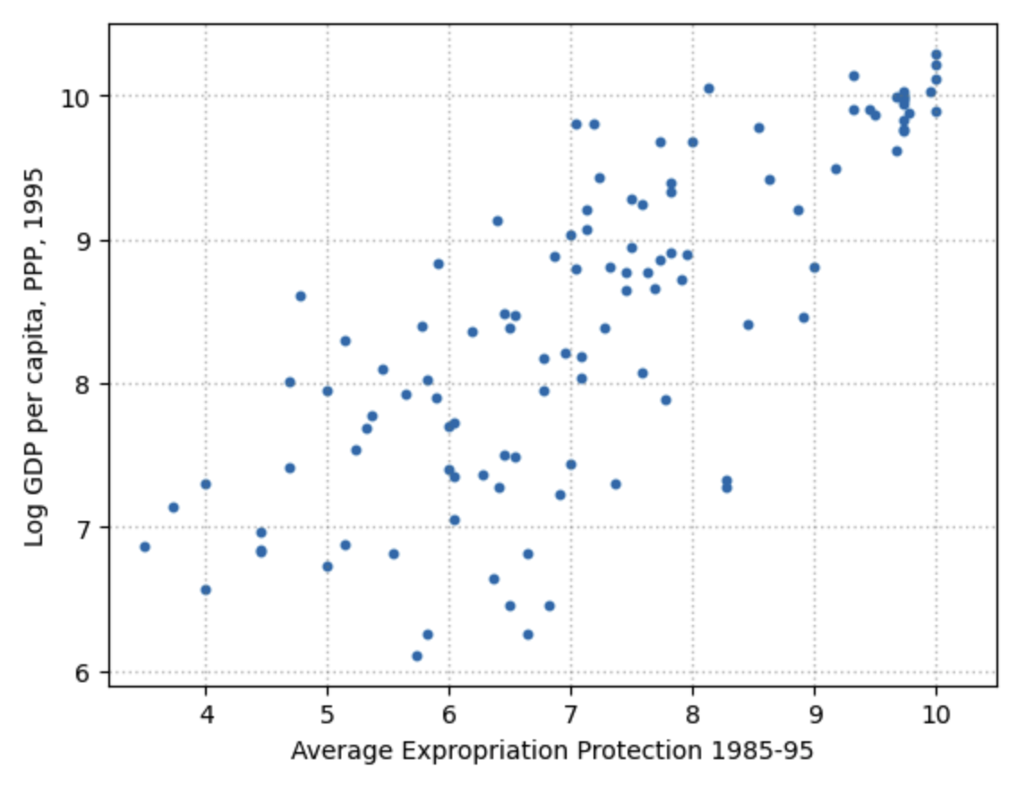
Fig. 12.2 Scatterplot of average expropriation protection \(avexpr\) and log GDP per capita \(logpgp95\) for each country

The plot shows a fairly strong positive relationship between protection against expropriation and log GDP per capita. Specifically, if higher protection against expropriation is a measure of institutional quality, then better institutions appear to be positively correlated with better economic outcomes (higher GDP per capita).

12.3.2. Cross tabulated data Description

Cross tabulation is a set of descriptive statics by groupings of the data. In R and Python, this is done with a powerful .groupby command. What if we thought that the relationship between protection against expropriation avexpr and logpgp95 were different for countries whose abbreviation started with A-M versus countries whose abbreviation started with N-Z?

# Create AtoM variable that = 1 if the first letter of the abbreviation is in
# A to M and = 0 if it is in N to Z
df1["AtoM"] = 0
df1["AtoM"][
    df1["shortnam"].str[0].isin([
        'A','B','C','D','E','F','G','H','I','J','K','L','M'
    ])
] = 1

# Describe the data
df1.groupby("AtoM").describe()

/tmp/ipykernel_2763/3993614049.py:4: SettingWithCopyWarning: 
A value is trying to be set on a copy of a slice from a DataFrame

See the caveats in the documentation: https://pandas.pydata.org/pandas-docs/stable/user_guide/indexing.html#returning-a-view-versus-a-copy
  df1["AtoM"][

	euro1900								excolony		...	loghjypl		baseco
	count	mean	std	min	25%	50%	75%	max	count	mean	...	75%	max	count	mean	std	min	25%	50%	75%	max
AtoM
0	55.0	28.449091	40.994987	0.0	0.0	1.0	50.0	100.0	58.0	0.689655	...	-0.870507	0.000000	24.0	1.0	0.0	1.0	1.0	1.0	1.0	1.0
1	99.0	31.586870	43.310207	0.0	0.0	2.0	99.5	100.0	104.0	0.653846	...	-0.763590	-0.014099	40.0	1.0	0.0	1.0	1.0	1.0	1.0	1.0

2 rows × 96 columns

Another way we could do this that is more readable that the output above is to just describe the data in two separate commands in which we restrict the data to the two separate groups.

df1[df1["AtoM"]==1].describe()

	euro1900	excolony	avexpr	logpgp95	cons1	cons90	democ00a	cons00a	extmort4	logem4	loghjypl	baseco	AtoM
count	99.000000	104.000000	74.000000	95.000000	55.000000	55.000000	55.000000	57.000000	58.000000	58.000000	75.000000	40.0	104.0
mean	31.586870	0.653846	7.204545	8.381995	3.672727	3.654546	1.236364	2.000000	220.015854	4.534877	-1.701214	1.0	1.0
std	43.310207	0.478047	1.854914	1.104331	2.373110	2.374386	2.624413	1.982062	431.900574	1.347500	1.119577	0.0	0.0
min	0.000000	0.000000	1.636364	6.109248	1.000000	1.000000	0.000000	1.000000	2.550000	0.936093	-3.540459	1.0	1.0
25%	0.000000	0.000000	6.045455	7.417576	1.000000	2.000000	0.000000	1.000000	68.075005	4.220586	-2.789016	1.0	1.0
50%	2.000000	1.000000	7.204545	8.301521	3.000000	3.000000	0.000000	1.000000	81.599998	4.400960	-1.560648	1.0	1.0
75%	99.500000	1.000000	8.613637	9.366871	7.000000	6.500000	1.000000	1.000000	259.889984	5.559247	-0.763590	1.0	1.0
max	100.000000	1.000000	10.000000	10.288750	7.000000	7.000000	10.000000	7.000000	2940.000000	7.986165	-0.014099	1.0	1.0

df1[df1["AtoM"]==0].describe()

	euro1900	excolony	avexpr	logpgp95	cons1	cons90	democ00a	cons00a	extmort4	logem4	loghjypl	baseco	AtoM
count	55.000000	58.000000	47.000000	53.000000	33.000000	33.000000	32.000000	34.000000	29.000000	29.000000	48.000000	24.0	59.0
mean	28.449091	0.689655	6.849130	8.160035	3.454545	3.606061	1.000000	1.617647	222.747574	4.718197	-1.777811	1.0	0.0
std	40.994987	0.466675	1.718516	1.103215	2.513599	2.317588	2.527271	1.517867	374.625153	1.223847	1.035098	0.0	0.0
min	0.000000	0.000000	3.000000	6.253829	1.000000	1.000000	0.000000	1.000000	8.550000	2.145931	-3.540459	1.0	0.0
25%	0.000000	0.000000	5.818182	7.279319	1.000000	1.000000	0.000000	1.000000	71.000000	4.262680	-2.710639	1.0	0.0
50%	1.000000	1.000000	6.863636	8.107720	3.000000	3.000000	0.000000	1.000000	140.000000	4.941642	-1.595533	1.0	0.0
75%	50.000000	1.000000	7.659091	8.885994	7.000000	7.000000	1.000000	1.000000	240.000000	5.634789	-0.870507	1.0	0.0
max	100.000000	1.000000	10.000000	10.215740	7.000000	7.000000	10.000000	7.000000	2004.000000	7.602901	0.000000	1.0	0.0

Let’s make two scatterplots to see with our eyes if there seems to be a difference in the relationship.

# Plot the scatterplot of the relationship for the countries for which the first
# letter of the abbreviation is between A to M
plt.scatter(
  x=df1[df1["AtoM"]==1]["avexpr"], y=df1[df1["AtoM"]==1]["logpgp95"], s=10
)
plt.xlim((3.2, 10.5))
plt.ylim((5.9, 10.5))
plt.title("Scatterplot of average expropriation protection and log GDP per " +
          "capita \n for each country, first letter in A-M")
plt.xlabel(r'Average Expropriation Protection 1985-95')
plt.ylabel(r'Log GDP per capita, PPP, 1995')
plt.grid(color='gray', linestyle=':', linewidth=1, alpha=0.5)
plt.show()

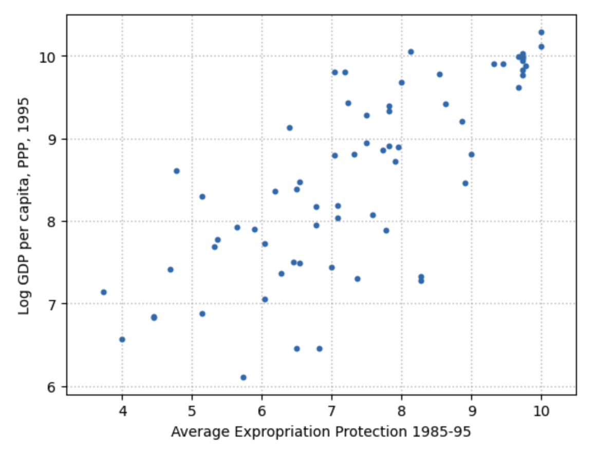
Fig. 12.3 Scatterplot of average expropriation protection \(avexpr\) and log GDP per capita \(logpgp95\) for each country, first letter in A-M

# Plot the scatterplot of the relationship for the countries for which the first
# letter of the abbreviation is between N to Z
plt.scatter(
  x=df1[df1["AtoM"]==0]["avexpr"], y=df1[df1["AtoM"]==0]["logpgp95"], s=10
)
plt.xlim((3.2, 10.5))
plt.ylim((5.9, 10.5))
plt.title("Scatterplot of average expropriation protection and log GDP per " +
          "capita \n for each country, first letter in N-Z")
plt.xlabel(r'Average Expropriation Protection 1985-95')
plt.ylabel(r'Log GDP per capita, PPP, 1995')
plt.grid(color='gray', linestyle=':', linewidth=1, alpha=0.5)
plt.show()

Fig. 12.4 Scatterplot of average expropriation protection \(avexpr\) and log GDP per capita \(logpgp95\) for each country, first letter in N-Z

12.4. Basic Understanding of Linear Regression

12.4.1. Example: Acemoglu, et al (2001)

Given the plots in Figure 12.2, Figure 12.3, and Figure 12.4 above, choosing a linear model to describe this relationship seems like a reasonable assumption.

We can write a model as:

(12.1)\[ logpgp95_i = \beta_0 + \beta_1 avexpr_i + u_i\]

where:

• \(\beta_0\) is the intercept of the linear trend line on the \(y\)-axis

• \(\beta_1\) is the slope of the linear trend line, representing the marginal effect of protection against risk on log GDP per capita

• \(u_i\) is a random error term (deviations of observations from the linear trend due to factors not included in the model)

Visually, this linear model involves choosing a straight line that best fits the data according to some criterion, as in the following plot (Figure 2 in [Acemoglu et al., 2001]).

import numpy as np

# Dropping NA's is required to use numpy's polyfit
df1_subset = df1.dropna(subset=['logpgp95', 'avexpr'])
# df1_subset.describe()

# Use only 'base sample' for plotting purposes (smaller sample)
df1_subset = df1_subset[df1_subset['baseco'] == 1]
# df1_subset.describe()

X = df1_subset['avexpr']
y = df1_subset['logpgp95']
labels = df1_subset['shortnam']

# Replace markers with country labels
plt.scatter(X, y, marker='')

for i, label in enumerate(labels):
    plt.annotate(label, (X.iloc[i], y.iloc[i]))

# Fit a linear trend line
plt.plot(np.unique(X),
         np.poly1d(np.polyfit(X, y, 1))(np.unique(X)),
         color='black')

plt.xlabel('Average Expropriation Protection 1985-95')
plt.ylabel('Log GDP per capita, PPP, 1995')
plt.xlim((3.2, 10.5))
plt.ylim((5.9, 10.5))
plt.title('OLS relationship between expropriation risk and income (Fig. 2 from Acemoglu, et al 2001)')
plt.show()

Fig. 12.5 OLS relationship between expropropriation risk and income (Fig. 2 from Acemoglu, et al, 2001)

The most common technique to estimate the parameters (\(\beta\)‘s) of the linear model is Ordinary Least Squares (OLS). As the name implies, an OLS model is solved by finding the parameters that minimize the sum of squared residuals.

(12.2)\[ \hat{\beta}_{OLS} = \beta : \quad \min_{\beta}\: u(X|\beta_0,\beta_1)^T \: u(X|\beta_0,\beta_1)\]

where \(\hat{u}_i\) is the difference between the dependent variable observation \(logpgp95_i\) and the predicted value of the dependent variable \(\beta_0 + \beta_1 avexpr_i\). To estimate the constant term \(\beta_0\), we need to add a column of 1’s to our dataset (consider the equation if \(\beta_0\) was replaced with \(\beta_0 x_i\) where \(x_i=1\)).

df1['const'] = 1

Now we can construct our model using the statsmodels module and the OLS method. We will use pandas DataFrames with statsmodels. However, standard arrays can also be used as arguments.

!pip install --upgrade statsmodels

import statsmodels.api as sm

reg1 = sm.OLS(endog=df1['logpgp95'], exog=df1[['const', 'avexpr']], missing='drop')
type(reg1)

statsmodels.regression.linear_model.OLS

So far we have simply constructed our model. The statsmodels.regression.linear_model.OLS is simply an object specifying dependent and independent variables, as well as instructions about what to do with missing data. We need to use the .fit() method to obtain OLS parameter estimates \(\hat{\beta}_0\) and \(\hat{\beta}_1\). This method calculates the OLS coefficients according to the minimization problem in (12.2).

results = reg1.fit()
type(results)

statsmodels.regression.linear_model.RegressionResultsWrapper

We now have the fitted regression model stored in results (see statsmodels.regression.linear_model.RegressionResultsWrapper). The results from the reg1.fit() command is a regression results object with a lot of information, similar to the results object of the scipy.optimize.minimize() function we worked with in the Maximum Likelihood Estimation and Generalized Method of Moments Estimation chapters.

To view the OLS regression results, we can call the .summary() method.

[Note that an observation was mistakenly dropped from the results in the original paper (see the note located in maketable2.do from Acemoglu’s webpage), and thus the coefficients differ slightly.]

print(results.summary())

                            OLS Regression Results                            
==============================================================================
Dep. Variable:               logpgp95   R-squared:                       0.611
Model:                            OLS   Adj. R-squared:                  0.608
Method:                 Least Squares   F-statistic:                     171.4
Date:                Fri, 15 Dec 2023   Prob (F-statistic):           4.16e-24
Time:                        23:35:33   Log-Likelihood:                -119.71
No. Observations:                 111   AIC:                             243.4
Df Residuals:                     109   BIC:                             248.8
Df Model:                           1                                         
Covariance Type:            nonrobust                                         
==============================================================================
                 coef    std err          t      P>|t|      [0.025      0.975]
------------------------------------------------------------------------------
const          4.6261      0.301     15.391      0.000       4.030       5.222
avexpr         0.5319      0.041     13.093      0.000       0.451       0.612
==============================================================================
Omnibus:                        9.251   Durbin-Watson:                   1.689
Prob(Omnibus):                  0.010   Jarque-Bera (JB):                9.170
Skew:                          -0.680   Prob(JB):                       0.0102
Kurtosis:                       3.362   Cond. No.                         33.2
==============================================================================

Notes:
[1] Standard Errors assume that the covariance matrix of the errors is correctly specified.

We can get individual items from the results, which are saved as attributes.

print(dir(results))
print("")
print("Degrees of freedom residuals:", results.df_resid)
print("")
print("Estimated coefficients:")
print(results.params)
print("")
print("Standard errors of estimated coefficients:")
print(results.bse)

['HC0_se', 'HC1_se', 'HC2_se', 'HC3_se', '_HCCM', '__class__', '__delattr__', '__dict__', '__dir__', '__doc__', '__eq__', '__format__', '__ge__', '__getattribute__', '__gt__', '__hash__', '__init__', '__init_subclass__', '__le__', '__lt__', '__module__', '__ne__', '__new__', '__reduce__', '__reduce_ex__', '__repr__', '__setattr__', '__sizeof__', '__str__', '__subclasshook__', '__weakref__', '_abat_diagonal', '_cache', '_data_attr', '_data_in_cache', '_get_robustcov_results', '_get_wald_nonlinear', '_is_nested', '_transform_predict_exog', '_use_t', '_wexog_singular_values', 'aic', 'bic', 'bse', 'centered_tss', 'compare_f_test', 'compare_lm_test', 'compare_lr_test', 'condition_number', 'conf_int', 'conf_int_el', 'cov_HC0', 'cov_HC1', 'cov_HC2', 'cov_HC3', 'cov_kwds', 'cov_params', 'cov_type', 'df_model', 'df_resid', 'diagn', 'eigenvals', 'el_test', 'ess', 'f_pvalue', 'f_test', 'fittedvalues', 'fvalue', 'get_influence', 'get_prediction', 'get_robustcov_results', 'info_criteria', 'initialize', 'k_constant', 'llf', 'load', 'model', 'mse_model', 'mse_resid', 'mse_total', 'nobs', 'normalized_cov_params', 'outlier_test', 'params', 'predict', 'pvalues', 'remove_data', 'resid', 'resid_pearson', 'rsquared', 'rsquared_adj', 'save', 'scale', 'ssr', 'summary', 'summary2', 't_test', 't_test_pairwise', 'tvalues', 'uncentered_tss', 'use_t', 'wald_test', 'wald_test_terms', 'wresid']

Degrees of freedom residuals: 109.0

Estimated coefficients:
const     4.626089
avexpr    0.531871
dtype: float64

Standard errors of estimated coefficients:
const     0.300575
avexpr    0.040621
dtype: float64

The powerful machine learning python package scikit-learn also has a linear regression function sklearn.linear_model.LinearRegression. It is very good at prediction, but it is harder to get things like standard errors that are valuable for inference.

12.4.2. What do coefficients and standard errors mean?

Go through cross terms and quadratic terms and difference-in-difference.

12.4.3. Interpreting results and output

From our results, we see that:

• the intercept \(\hat{\beta}_0=4.63\) (interpretation?)

• the slope \(\hat{\beta}_1=0.53\) (interpretation?)

• the positive \(\hat{\beta}_1>0\) parameter estimate implies that protection from expropriation has a positive effect on economic outcomes, as we saw in the figure.

• How would you quantitatively interpret the \(\hat{\beta}_1\) coefficient?

• What do the standard errors on the coefficients tell you?

• The p-value of 0.000 for \(\hat{\beta}_1\) implies that the effect of institutions on GDP is statistically significant (using \(p < 0.05\) as a rejection rule)

• The R-squared value of 0.611 indicates that around 61% of variation in log GDP per capita is explained by protection against expropriation

Using our parameter estimates, we can now write our estimated relationship as:

(12.3)\[ \hat{logpgp95}_i = 4.63 + 0.53 avexpr_i\]

This equation describes the line that best fits our data, as shown in Figure 12.5. We can use this equation to predict the level of log GDP per capita for a value of the index of expropriation protection (see Section Predicted values below).

12.4.4. Analysis of variance (ANOVA) output

The results .summary() method provides a lot of regression output. And the .RegressionResults object has much more as evidenced in the help page statsmodels.regression.linear_model.RegressionResults.

• The Df Residuals: 109 displays the degrees of freedom from the residual variance calculation. This equals the number of observations minus the number of regression coefficients, N-p=111-2. This is accessed with results.df_resid.

• The Df Model: 1 displays the degrees of freedom from the model variance calculation or from the regressors. This equals the number of regression coefficients minus one, p-1=2-1. This is accessed with results.df_model.

• One can specify robust standard errors in their regression. The robust option is specified in the .fit() command. You can specify three different types of robust standard errors using the .fit(cov_type='HC1'), .fit(cov_type='HC2'), or .fit(cov_type='HC3') options.

• You can do clustered standard errors if you have groups labeled in a variable called mygroups by using the .fit(cov_type='cluster', cov_kwds={'groups': mygroups}).

• R-squared is a measure of fit of the overall model. It is \(R^2=1 - SSR/SST\) where \(SST\) is the total variance of the dependent variable (total sum of squares), and \(SSR\) is the sum of squared residuals (variance of the residuals). Another expresion is the sum of squared predicted values over the total sum of squares \(R^2= SSM/SST\), where \(SSM\) is the sum of squared predicted values. This is accessed with results.rsquared.

• Adjusted R-squared is a measure of fit of the overall model that penalizes extra regressors. A property of the R-squared in the previous bullet is that it always increases as you add more explanatory variables. This is accessed with results.rsquared_adj.

12.4.5. F-test and log likelihood test

• The F-statistic is the statistic from an F-test of the joint hypothesis that all the coefficients are equal to zero. The value of the F-statistic is distributed according to the F-distribution \(F(d1,d2)\), where \(d1=p-1\) and \(d2=N-p\).

• The Prob (F-statistic) is the probability that the null hypothesis of all the coefficients being zero is true. In this case, it is really small.

• Log-likelihood is the sum of the log pdf values of the errors given their being normally distributed with mean 0 and standard deviation implied by the OLS estimates.

12.4.6. Inference on individual parameters

• The estimated coefficients of the linear regression are reported in the results.params vector object (pandas Series).

• The standard error on each estimated coefficient is reported in the summary results column entitled std err. These standard errors are reported in the results.bse vector object (pandas Series).

• The “t” column is the \(t\) test statistic. It is the value in the support of the students-T distribution that is equivalent to the estimated coefficient if the null-hypothesis were true that the estimated coefficient were 0.

• The reported p-value is the probability of a two-sided t-test that gives the probability that the estimated coefficient is greater than its estimated value if the true value were 0. A more intuitive interpretation is the probability of seeing that estimated value if the null hypothesis were true. We usually reject the null hypothesis if the p-value is lower than 0.05.

• The summary results report the 95% two-sided confidence interval for the estimated value.

12.4.7. Predicted values

We can obtain an array of predicted \(logpgp95_i\) for every value of \(avexpr_i\) in our dataset by calling .predict() on our results. Let’s first get the predicted value for the average country in the dataset.

mean_expr = np.mean(df1['avexpr'])
mean_expr

7.066491

print(results.params)

const     4.626089
avexpr    0.531871
dtype: float64

predicted_logpdp95 = 4.63 + 0.53 * mean_expr
print(predicted_logpdp95)

8.375240297317506

An easier (and more accurate) way to obtain this result is to use .predict() and set \(constant=1\) and \(avexpr_i=\) mean_expr.

results.predict(exog=[1, mean_expr])

array([8.38455358])

Plotting the predicted values against \(avexpr_i\) shows that the predicted values lie along the linear line that we fitted below in Figure 12.6. The observed values of \(logpgp95_i\) are also plotted for comparison purposes.

# Drop missing observations from whole sample
df1_plot = df1.dropna(subset=['logpgp95', 'avexpr'])

# Plot predicted values. alpha is a blending value between 0 (transparent) and 1 (opaque)
plt.scatter(df1_plot['avexpr'], results.predict(), alpha=0.5, label='predicted')

# Plot observed values
plt.scatter(df1_plot['avexpr'], df1_plot['logpgp95'], alpha=0.5, label='observed')

plt.legend()
plt.title('OLS predicted values')
plt.xlabel('Average Expropriation Protection 1985-95')
plt.ylabel('Log GDP per capita, PPP, 1995')
plt.show()

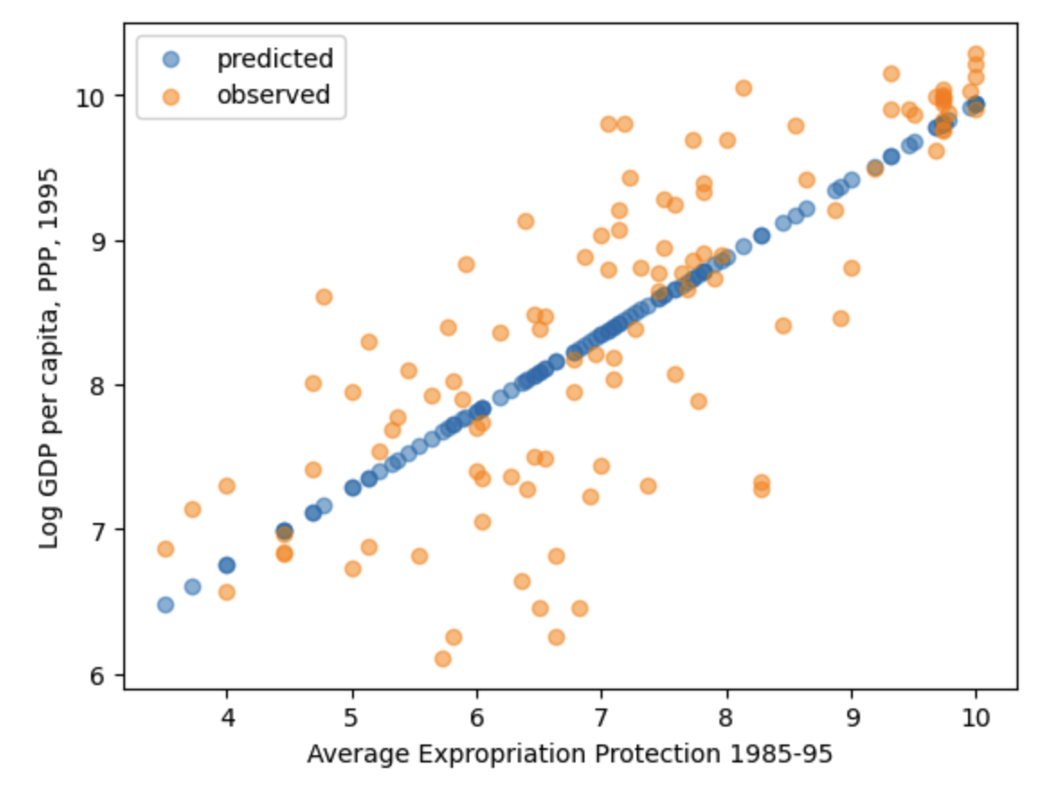
Fig. 12.6 OLS predicted values for Acemoglu, et al, 2001 data

12.5. Basic extensions of linear regression

• Instrumental variables (omitted variable bias)

• Logistic regression

• Multiple equation models

• Panel data

• Time series data

• Vector autoregression

12.6. Exercises

Exercise 12.1 (Multiple linear regression)

For this problem, you will use the 397 observations from the Auto.csv dataset in the /data/basic_empirics/ folder of the repository for this book.[2] This dataset includes 397 observations on the following variables:

• mpg: miles per gallon

• cylinders: number of cylinders

• displacement: engine displacement (cubic inches)

• horsepower: engine horsepower

• weight: vehicle weight (lbs.)

• acceleration: time to accelerate from 0 to 60 mph (sec.)

• year: vehicle year

• origin: origin of car (1=American, 2=European, 3=Japanese)

• name: vehicle name

1. Import the data using the pandas.read_csv() function. Look for characters that seem out of place that might indicate missing values. Replace them with missing values using the na_values=... option.

2. Create descriptive statistics for each of the numerical variables (count, mean, standard deviation, min, 25%, 50%, 75%, max). How do you interpret the descriptive statistics on the origin variable? What might be a better way to report descriptive statistics for this categorical variable?

3. Produce a scatterplot matrix which includes all of the numerical variables mpg, cylinders, displacement, horsepower, weight, acceleration, year, origin. Call your DataFrame of numerical variables df_numer. [Use the pandas scatterplot function in the code block below.]

from pandas.plotting import scatter_matrix

scatter_matrix(df_numer, alpha=0.3, figsize=(6, 6), diagonal='kde')

4. Compute the correlation matrix for the numerical variables (\(8\times 8\)) using the pandas.DataFrame.corr() method.

5. What is wrong with estimating the following linear regression model? How would you fix this problem? (Hint: There is an issue with one of the variables.)

   \[\begin{equation*} \begin{split} mpg_i &= \beta_0 + \beta_1 cylinders_i + \beta_2 displacement_i + \beta_3 horsepower_i + ... \\ &\qquad \beta_4 weight_i + \beta_5 acceleration_i + \beta_6 year_i + \beta_7 origin_i + u_i \end{split} \end{equation*}\]

6. Estimate the following multiple linear regression model of \(mpg_i\) on all other numerical variables, where \(u_i\) is an error term for each observation, using Python’s statsmodels.api.OLS() function, with indicator variables created for two out of the three origin categories (2=European, 3=Japanese).

   \[\begin{equation*} \begin{split} mpg_i &= \beta_0 + \beta_1 cylinders_i + \beta_2 displacement_i + \beta_3 horsepower_i + ... \\ &\qquad \beta_4 weight_i + \beta_5 acceleration_i + \beta_6 year_i + ...\\ &\qquad \beta_7 european_i + \beta_8 japanese_i + u_i \end{split} \end{equation*}\]

   • Which of the coefficients is statistically significant at the 1% level?

   • Which of the coefficients is NOT statistically significant at the 10% level?

   • Give an interpretation in words of the estimated coefficient \(\hat{\beta}_6\) on \(year_i\) using the estimated value of \(\hat{\beta}_6\).

7. Looking at your scatterplot matrix from part (2), what are the three variables that look most likely to have a nonlinear relationship with \(mpg_i\)?

   • Estimate a new multiple regression model by OLS in which you include squared terms on the three variables you identified as having a nonlinear relationship to \(mpg_i\) as well as a squared term on \(acceleration_i\).

   • Report your adjusted R-squared statistic. Is it better or worse than the adjusted R-squared from part (4)?

   • What happened to the statistical significance of the \(displacement_i\) variable coefficient and the coefficient on its squared term?

   • What happened to the statistical significance of the cylinders variable?

8. Using the regression model from part (6) and the .predict() function, what would be the predicted miles per gallon \(mpg\) of a car with 6 cylinders, displacement of 200, horsepower of 100, a weight of 3,100, acceleration of 15.1, model year of 1999, and origin of 1 (American)?

12.7. Footnotes

The footnotes from this chapter.

---

[1]

For a tutorial on using Python’s Pandas package, see the Pandas chapter of this online book.

[2]

The Auto.csv dataset comes from [James et al., 2017] (ch. 3) and is also available at http://www-bcf.usc.edu/~gareth/ISL/data.html.